
4.1 AnoPrimer, advanced: qPCR, copy number and SNP-genotyping assays
Theme: Tools & technology
On Days 2 and 3 you built the first half of your gene dossier. Your candidate genes are
overexpressed in the deltamethrin-selected Busia colony, they replicate across studies in
AnoExpress, and in wild Ugandan mosquitoes you looked for the CNVs, missense variants and
selection signals that might explain that overexpression. The Busia 2016 cohort
(UG-E_Busia_gamb_2016_Q2) carries four selection signals, and you picked candidate SNPs on
the swept haplotypes.
None of that helps a control programme until somebody can measure it in a field insectary for a few cents per mosquito. Today we build the assays.
Our worked example is CYP6AA1 (AGAP002862), which sits at the head of the 2R Cyp6aa/p cluster. It is a good example because the interesting thing about it in East Africa is not a single mutation but a haplotype of three linked changes - a Cyp6aa1 duplication, the Cyp6p4-I236M substitution, and a Ty3/Gypsy (“ZZB”) transposable element insertion - which arose near the Kenya-Uganda border, spread to the DRC and Tanzania, and predicts both deltamethrin resistance and the benefit of PBO nets (Njoroge et al. 2022). That paper built LNA probe diagnostics for all three. Between them, those three markers need three different assay designs, which is exactly the range this module covers:
| # | Question | Assay | AnoPrimer assay_type |
|---|---|---|---|
| a | Is CYP6AA1 overexpressed in these mosquitoes? | RT-qPCR on cDNA | cDNA primers |
| b | How many copies of Cyp6aa1 does this mosquito have? | copy-number qPCR on gDNA | gDNA primers |
| c | Does it carry Cyp6p4-I236M? | probe genotyping assay | gDNA primers + probe |
| d | Will any of it work in Busia? | Ag3 frequencies under every oligo | (all of the above) |
We use AnoPrimer, which wraps primer3-py and the malariagen_data API, so every candidate oligo can be scored against Ag3 variation before you spend money on it.

Learning objectives
At the end of this module you will be able to:
Choose the right AnoPrimer assay type (
gDNA primers,cDNA primers,gDNA primers + probe,probe) for a surveillance question.Design RT-qPCR primers that span an exon-exon junction, and check them against a close paralogue.
Design a copy-number qPCR assay, and choose a single-copy reference locus using Ag3 CNV data.
Explain how hydrolysis (TaqMan) probes and allele-specific LNA probes genotype a SNP, and why locked bases raise Tm and sharpen mismatch discrimination.
Score your own oligos against Ag3 variation in the Busia cohort, and run in-silico specificity checks, to decide what to order.
A ten-minute recap
This module assumes the PAMCA workshop 6 module on AnoPrimer. If any of the following is hazy, skim it now - we will not re-teach it:
W6-M4: AnoPrimer - primer design in Anopheles gambiae: the stages of PCR; SYBR green versus probes; why SNPs in primer binding sites cause null alleles and biased Cq values; gDNA primers for ace1-G280S and RT-qPCR primers for COEAE2F.
The three things we build on directly:
Primer rules of thumb. 17-24 bases, Tm 57-63 degrees C (ideally 60), GC 30-70%, no runs of four or more Gs, no strong self- or cross-complementarity. primer3 enforces all of this for you.
SNPs matter most at the 3’ end. A mismatch in the last five bases sits in the polymerase active site and can shift Cq by 5-7 cycles, or abolish amplification. In An. gambiae s.l. you find a SNP roughly every other accessible base, so this is not a rare event.
AnoPrimer’s job is to hand primer3 the right template - genomic sequence for gDNA assays, concatenated exons with junctions marked for cDNA assays - and then paint Ag3 allele frequencies onto every base of every candidate oligo.
The four assay types
assay_type | Template | Designs | Typical use |
|---|---|---|---|
gDNA primers | genomic sequence around a position | forward + reverse | endpoint PCR, Sanger, copy-number qPCR, amplicon panels |
cDNA primers | exons concatenated, junctions marked | forward + reverse | RT-qPCR for gene expression |
gDNA primers + probe | genomic sequence around a position | forward + reverse + internal probe | TaqMan / LNA genotyping |
probe | genomic sequence around a position | internal probe only | adding a probe to primers you already have |
gDNA and probe targets are a contig:position string such as '2R:28497967'.
cDNA primers take a transcript identifier such as 'AGAP002862-RA'.
Setup
Pinned versions. anoprimer pulls in primer3-py, gget, seaborn and openpyxl, so we
only pin the two packages that matter. Installation takes a couple of minutes on Colab.
%pip install -q --no-warn-conflicts anoprimer==2.0.8 malariagen_data==15.9.0import warnings
warnings.simplefilter(action="ignore", category=Warning)
import AnoPrimer
import malariagen_data
import numpy as np
import pandas as pd
pd.set_option("display.max_columns", 30)
%matplotlib inline
%config InlineBackend.figure_format = "retina"
print("AnoPrimer 2.0.8 | malariagen_data", malariagen_data.__version__)A warning about a missing Google Cloud project ID can safely be ignored. AnoPrimer opens its
own Ag3() client internally, so there is nothing to configure; note that the MalariaGEN
resources are subject to their
terms of use.
Your candidate genes, SNP and cohort
Replace these with the genes you were assigned on Day 2 (data/candidate-genes.tsv) and the
SNP you chose on Day 3. The defaults are CYP6AA1 and GSTE4, and the Cyp6p4-I236M mutation.
# Replace with the genes you were assigned on Day 2 (see data/candidate-genes.tsv)
CANDIDATE_GENES = ["AGAP002862", "AGAP009193"]  # CYP6AA1, GSTE4

# Replace with a SNP you found on a swept haplotype on Day 3, as 'contig:position' (AgamP4).
# NB: AnoPrimer and malariagen_data use 1-based positions. The Ag-vampIR BED file, like all
# BED files, is 0-based, so the same SNP appears there as 2R 28497966 28497967.
CANDIDATE_SNP = "2R:28497967"  # Cyp6p4-I236M, on the 2R Cyp6aa/p sweep
CANDIDATE_SNP_NAME = "Cyp6p4-I236M"
CANDIDATE_SNP_ALT = "C"  # the resistance allele: 2R:28497967 G>C

# The Busia cohort. Sample set 1178-VO-UG-LAWNICZAK-VMF00025 holds the 24 An. gambiae of the
# UG-E_Busia_gamb_2016_Q2 atlas cohort you worked with on Day 3.
BUSIA_SAMPLE_SETS = "1178-VO-UG-LAWNICZAK-VMF00025"
BUSIA_QUERY = "cohort_admin2_quarter == 'UG-E_Busia_gamb_2016_Q2'"

# AnoPrimer wants transcripts, not genes, for cDNA assays. -RA is the only transcript of both
# default genes; check the gff if one of yours has several.
CANDIDATE_TRANSCRIPTS = [f"{g}-RA" for g in CANDIDATE_GENES]
CANDIDATE_TRANSCRIPTS
(a) RT-qPCR primers for CYP6AA1
Why the design differs from a gDNA assay
Your Day 2 evidence is expression. To confirm it in new mosquitoes the cheapest assay is RT-qPCR: extract RNA, make cDNA, and measure how many cycles each sample takes to cross a fluorescence threshold (its Cq).
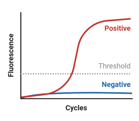
Four constraints, all different from a genotyping assay.
1. The primers must not amplify genomic DNA. RNA extractions carry residual gDNA. A primer
pair sitting inside a single exon will amplify that gDNA happily and inflate apparent
expression. The standard fix is to make one primer span an exon-exon junction: the junction
exists only in mature mRNA, so gDNA cannot template it. AnoPrimer does this by concatenating
the exons of your transcript, recording the junctions, and passing them to primer3 as
SEQUENCE_OVERLAP_JUNCTION_LIST (cDNA_exon_junction=True, the default). This is the single
most common flaw in published mosquito RT-qPCR assays.
2. Short amplicons, 60-120 bp. Short products amplify with near-perfect efficiency, tolerate partly degraded RNA and cycle quickly. There is no benefit to a long product, because you never look at it directly.
3. Efficiency. A perfect reaction doubles the product every cycle (efficiency 2, or 100%). You measure it with a dilution series of cDNA, fitting Cq against log(dilution); you want 90-110% with R-squared above 0.98. Lower usually means secondary structure, a dimer, or a SNP under a primer. The familiar delta-delta-Cq calculation assumes target and reference assays are both near 100%, so an unmeasured efficiency is an unquantified bias.
4. Reference genes. Cq alone measures how much cDNA you loaded. Expression is always a ratio to reference (“housekeeping”) genes that do not change between your conditions. Njoroge et al. (2022) measured Cyp6aa1, Cyp6p4 and Cyp6p3 by SYBR green qPCR normalised to S7 ribosomal protein (AGAP010592) and elongation factor (AGAP005128) - a reasonable default pair for An. gambiae. Validate two or three in your own samples, and never use a reference gene that sits in a duplicated or swept region (we check this below).
primers = AnoPrimer.design_primers(
    species="gambiae_sl",
    assay_type="cDNA primers",
    assay_name=CANDIDATE_TRANSCRIPTS[0],
    target=CANDIDATE_TRANSCRIPTS[0],
    min_amplicon_size=60,
    max_amplicon_size=120,
    n_primer_pairs=6,
    primer_parameters="default",   # or 'stringent', 'relaxed', or your own dict
    cDNA_exon_junction=True,       # keep True for qPCR
)

primers.df
Read the output from the top:
Exon junctions for ...lists the junctions, first in cDNA coordinates then in genome coordinates.AGAP002862-RAhas a single junction, at cDNA position 783 (2R:28481359). With only one junction primer3 has a narrow window to work in, and if it returns nothing that is usually why - the fix isprimer_parameters='relaxed'or a wider amplicon range. A single-exon gene cannot be designed this way at all; there you need a DNase treatment and a no-reverse-transcriptase control instead.primer_forward_span/primer_reverse_spanare genome coordinates. A junction-spanning primer has a span covering two exons, so it looks far wider than the primer is long (for example2R:28481349-28481474for a 23-mer). That is how you spot it.primer_pair_product_sizeis measured on the cDNA, which is what your product will be.
The three built-in parameter sets: default (Tm 57-63, size 17-24), stringent (adds
PRIMER_PAIR_MAX_DIFF_TM = 2 and tight self-complementarity limits - use it if the assay will
be multiplexed) and relaxed (Tm 55-64, size 18-27, for awkward templates). You can also pass
a dictionary of any primer3 global parameters.
The paralogue problem
CYP6AA1 has an immediate neighbour, CYP6AA2 (AGAP013128, 2R:28483301-28484921), a close
paralogue about 700 bp away, and eight more Cyp6 genes follow it along the cluster. Paralogues
are the classic way an expression assay goes quietly wrong: the primers amplify both genes, and
you report the sum as if it were your gene.
Neither primer3 nor the Ag3 frequency plot will tell you this, because both look only at your target region. Check it directly: pull the paralogue’s sequence and look for your primer, its reverse complement, and - more sensitively - its 3’-terminal 12 bases, which are what the polymerase needs in order to extend.
def reverse_complement(seq):
    return seq[::-1].translate(str.maketrans("ACGT", "TGCA"))


def check_against_paralogue(results, region, label):
    """Look for each oligo (and its 3' end) in another gene's genomic sequence."""
    paralogue = "".join(
        results.data_resource.genome_sequence(region=region).compute().astype(str)
    )
    rows = []
    for pair in results.df.columns:
        for oligo in ["forward", "reverse"]:
            seq = results.df[pair].loc[f"primer_{oligo}_sequence"]
            three_prime = seq[-12:]
            rows.append(
                dict(
                    pair=pair,
                    oligo=oligo,
                    sequence=seq,
                    full_match=(seq in paralogue) or (reverse_complement(seq) in paralogue),
                    three_prime_match=(three_prime in paralogue)
                    or (reverse_complement(three_prime) in paralogue),
                )
            )
    out = pd.DataFrame(rows)
    out.insert(0, "paralogue", label)
    return out


check_against_paralogue(primers, "2R:28483301-28484921", "CYP6AA2 (AGAP013128)")
With the default parameters, pair 4’s reverse primer (AAGCTTCAACTCCACGACGG) matches
CYP6AA2 exactly - it would amplify both genes. Pairs 2, 4 and 6 have a 3’-terminal 12-mer
present in the paralogue, which is a weaker warning but still worth avoiding. Pairs 1, 3 and 5
are clean on this test.
This is an exact-string check, so it is a floor, not a ceiling: it finds identical stretches but not near-identical ones. Primer-BLAST restricted to An. gambiae (taxid 7165) is the proper version of this check, and the BLAT step later in this notebook is a quick approximation.
Checking the primers against Busia variation
.plot_primer_snp_frequencies() paints Ag3 allele frequencies onto every base of every oligo.
We restrict to the Busia cohort, because a primer that is clean genome-wide can still be
useless in the population you plan to survey.
primers.summarise_metadata(sample_sets=BUSIA_SAMPLE_SETS, sample_query=BUSIA_QUERY)snp_freqs = primers.plot_primer_snp_frequencies(
sample_sets=BUSIA_SAMPLE_SETS,
sample_query=BUSIA_QUERY,
)Each panel is one oligo, 5’ on the left and 3’ on the right, with the reference base on the x axis and the summed alternate allele frequency on the y. Grey points are invariant in this cohort, blue points segregating. Hover to see all four per-base frequencies, and read the Tm, GC and genomic span printed on the panel.
How to use it:
A blue point in the last five bases at the 3’ end: reject the pair.
A high-frequency alternate allele anywhere in the oligo: reject, or order a degenerate primer carrying both bases. A primer matching the reference at a site where the population is 90% alternate is a primer that mostly mismatches the mosquitoes you want to measure.
Low-frequency variants in the middle of a long primer: usually tolerable.
Everything grey: you are looking at 24 mosquitoes from one place and quarter. Widen the cohort before ordering (Exercise 2).
The returned dictionary lets you filter by rule rather than by eye.
# flag any segregating site in the 3'-most 5 bases of any oligo
rows = []
for pair, oligos in snp_freqs.items():
    for oligo, df in oligos.items():
        rows.append(
            dict(
                pair=pair,
                oligo=oligo,
                max_alt_freq=round(df["alt_frequency"].max(), 3),
                max_alt_freq_3prime=round(df.tail(5)["alt_frequency"].max(), 3),
                n_segregating=int((df["alt_frequency"] > 0).sum()),
            )
        )

pd.DataFrame(rows).sort_values(["max_alt_freq_3prime", "max_alt_freq"], ascending=False)
primers.plot_primer_locs(legend_loc="lower left")Grey boxes are exons of the transcript, numbered; black outlines are genes. Primers are drawn as arrows in the direction they extend, and a dotted arrow spans an exon-exon junction. At least one oligo of the pair you order must be dotted.
Exercise 1
Design RT-qPCR primers for your second candidate gene, check them against Busia variation, and choose the pair you would order. Record: which pair, which oligo spans the junction, the amplicon size, the highest alternate allele frequency in either oligo, and (if your gene has a close paralogue) the result of the paralogue check.
Show answer
primers2 = AnoPrimer.design_primers(
    species="gambiae_sl",
    assay_type="cDNA primers",
    assay_name=CANDIDATE_TRANSCRIPTS[1],
    target=CANDIDATE_TRANSCRIPTS[1],
    min_amplicon_size=60,
    max_amplicon_size=120,
    n_primer_pairs=6,
    primer_parameters="default",
)
primers2.evaluate_primers(
    sample_sets=BUSIA_SAMPLE_SETS, sample_query=BUSIA_QUERY, out_dir="."
)
primers2.to_csv("gste4.cDNA_primers.tsv", sep="\t")

# GSTE4 sits in the Gste cluster, so check its neighbours too
check_against_paralogue(primers2, "3R:28597000-28599000", "GSTE2 (AGAP009194)")
AGAP009193-RA (GSTE4) has a single exon junction, at cDNA position 452 (3R:28596400), and with the default parameters primer3 returns just one pair - a good illustration of how tight a single-junction design is. If you need alternatives, use primer_parameters='relaxed' or widen max_amplicon_size. GSTE4 lies in the Gste cluster next to GSTE2, GSTE3 and GSTE1, so the paralogue check matters here as much as it does for CYP6AA1.
# your answer here(b) A copy-number qPCR assay for the Cyp6aa1 duplication
Why copy number, and why gDNA
For CYP6AA1 in East Africa, the reason the gene is overexpressed is largely that there is more than one of it. Duplications raise transcript abundance without changing a single base of coding sequence, and they are common across the An. gambiae detoxification loci.
That makes the cheaper, more robust field assay a copy-number qPCR on genomic DNA. gDNA is far easier than RNA to collect, store and ship - no RNAlater, no cold chain, no worrying that expression changed while the mosquito sat in a tube.
First, confirm from Ag3 that the duplication is really there, and see which genes it covers.
ag3 = malariagen_data.Ag3()

cnv_freqs = ag3.gene_cnv_frequencies(
    region="2R:28,470,000-28,510,000",   # the Cyp6aa/p cluster
    cohorts="admin2_quarter",
    sample_sets=["3.0", "3.3", "3.8"],
    min_cohort_size=10,
)

busia_cols = [c for c in cnv_freqs.columns if "Busia" in c]
cnv_freqs.reset_index()[["gene_id", "gene_name", "cnv_type"] + busia_cols]
The amplification frequencies tell you where to put the assay. In Busia the Cyp6aa1 amplification is at 0.95 in 2016 and 1.00 by 2019, while Cyp6aa2 is at 0.30 and the Cyp6p genes lower still - the duplication is centred on Cyp6aa1, which is why the diagnostic targets that gene and not its neighbours. (Compare this with your Day 3 CNV work: the frequencies here are per-cohort amplification calls from the Ag3 CNV HMM.)
Designing it
Use gDNA primers: the intended template is genomic DNA, so the exon-junction trick would
actively break this assay. Target a position well inside Cyp6aa1, and keep the amplicon
short (80-150 bp) so the reaction is robust on crudely extracted field DNA.
cnv_primers = AnoPrimer.design_primers(
    species="gambiae_sl",
    assay_type="gDNA primers",
    assay_name="Cyp6aa1-copy-number",
    target="2R:28481500",         # inside AGAP002862 (2R:28,480,576-28,482,637)
    min_amplicon_size=80,
    max_amplicon_size=150,
    n_primer_pairs=4,
    primer_parameters="default",
)

cnv_primers.df
# the paralogue check matters even more here: Cyp6aa2 is 700 bp away and also amplified
check_against_paralogue(cnv_primers, "2R:28483301-28484921", "CYP6AA2 (AGAP013128)")Choosing the single-copy reference locus
Copy number is a ratio, so the assay is only as good as its denominator: a second qPCR on the same gDNA, at a locus you are confident is present in exactly two copies in your populations. Then, with efficiency near 100%,
delta_Cq      = Cq(target) - Cq(reference)
copy_number   = 2 * 2 ** -(delta_Cq - delta_Cq_of_a_known_2-copy_control)
which is the familiar delta-delta-Cq, with a known two-copy susceptible strain (Kisumu, say) as the calibrator.
The mistake to avoid is picking a reference locus that is itself variable in copy number. You can check any candidate against Ag3 before you commit.
candidate_refs = {
    "AGAP010592 (S7 ribosomal protein)": "3L:6,560,000-6,572,000",
    "AGAP005128 (elongation factor)": "2L:10,331,000-10,344,000",
}

for label, region in candidate_refs.items():
    freqs = ag3.gene_cnv_frequencies(
        region=region,
        cohorts="admin2_quarter",
        sample_sets=["3.0", "3.3", "3.8"],
        min_cohort_size=10,
    ).reset_index()
    cols = [c for c in freqs.columns if "Busia" in c]
    print(label)
    print(freqs[["gene_id", "gene_name", "cnv_type"] + cols].to_string(index=False), "\n")
S7 (AGAP010592) has no amplification or deletion calls in any Busia cohort, so it is a sound denominator. AGAP005128 shows low-frequency amplification (about 9% in 2017), which makes it a slightly risky one - fine as an RT-qPCR reference gene, where you normalise across many samples, but not ideal as the denominator of a per-mosquito copy-number ratio.
Design the reference assay the same way, then check both pairs against Busia variation.
ref_primers = AnoPrimer.design_primers(
    species="gambiae_sl",
    assay_type="gDNA primers",
    assay_name="S7-reference",
    target="3L:6566000",          # inside AGAP010592
    min_amplicon_size=80,
    max_amplicon_size=150,
    n_primer_pairs=4,
    primer_parameters="stringent",  # target and reference run side by side: match them tightly
)

ref_primers.df
_ = cnv_primers.plot_primer_snp_frequencies(
sample_sets=BUSIA_SAMPLE_SETS, sample_query=BUSIA_QUERY
)
_ = ref_primers.plot_primer_snp_frequencies(
sample_sets=BUSIA_SAMPLE_SETS, sample_query=BUSIA_QUERY
)Two extra points specific to copy-number assays:
Match the two assays’ efficiencies. The ratio is meaningless if target and reference amplify at different rates, which is why
stringent(withPRIMER_PAIR_MAX_DIFF_TM = 2) is a sensible choice when both reactions run on the same plate under one cycling programme.A null allele looks like a deletion. A SNP under a primer that suppresses amplification will read out as low copy number, not as a failed reaction. There is no no-template control that catches this - only the frequency check above.
(c) A probe genotyping assay for Cyp6p4-I236M
How a hydrolysis (TaqMan) probe works
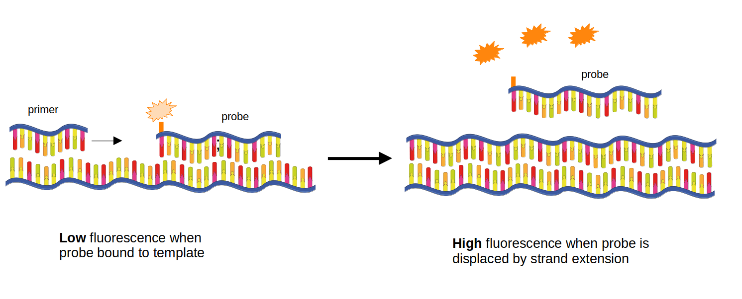
A hydrolysis probe is a short oligo binding inside the amplicon, between the primers, with a fluorophore at its 5’ end and a quencher at its 3’ end, so while intact it is dark. When the polymerase extends the forward primer it hydrolyses the probe; fluorophore and quencher separate, and the signal rises in proportion to the copies made. Unlike SYBR green, which stains any double-stranded DNA including primer dimers, fluorescence appears only if the probe’s own sequence was present - so the probe, not the primers, defines specificity.
Genotyping with two allele-specific probes
To genotype, design two probes over the same position, identical but for the SNP base, each with a different fluorophore (typically FAM and HEX/VIC). One reaction, two channels:
| FAM | HEX | Genotype |
|---|---|---|
| high | low | homozygous for the FAM allele |
| low | high | homozygous for the HEX allele |
| high | high | heterozygote |
| low | low | failed reaction, or a null allele from a SNP under a primer |
The discrimination is thermodynamic. At the annealing temperature the matched probe binds and the single-mismatch probe does not. That difference in stability is small, and smaller the longer the probe - one mismatch in 25 bases matters proportionally less than one in 12. So allele-specific probes want to be short, which drags their Tm below the annealing temperature, and a probe that does not bind reports nothing.
Which is what locked nucleic acids fix
An LNA base is a ribonucleotide whose ribose is bridged (2’-O, 4’-C methylene), locking the sugar in the conformation it takes up in a duplex. Because the base is pre-organised, binding costs less conformational entropy, so each LNA substitution raises duplex Tm by roughly 2-8 degrees C. Two consequences:
Short probes become usable. A 10-14 base probe with three or four LNAs reaches a Tm in the sixties, where the same length of plain DNA would melt below 40 degrees C.
Mismatch discrimination improves. A locked sugar makes the duplex less able to accommodate a distorted base pair, so the delta-Tm between matched and mismatched probe grows. Placing an LNA on, or immediately beside, the SNP maximises this.
This is how the kdr LNA assay genotypes Vgsc-995F and Vgsc-995S simultaneously with two short probes over adjacent codon positions, and it is the chemistry Njoroge et al. used for all three triple-mutant markers.
Practical notes. AnoPrimer deliberately keeps probe Tm limits wide
(PRIMER_INTERNAL_MIN_TM 45, MAX_TM 65) on the assumption that you will add LNA bases
afterwards and re-check. primer3 has no LNA thermodynamics, so that step happens outside
AnoPrimer, in IDT’s LNA oligo analyzer (free, needs
a login), where you move the locked positions and read off matched and mismatched Tm. Aim for a
matched Tm a few degrees above the annealing temperature, and a delta-Tm of at least 5-8
degrees C against the other allele.
Designing primers and a probe
gDNA primers + probe asks primer3 for a forward primer, a reverse primer and an internal
oligo, and AnoPrimer forces the internal oligo to overlap the target position (it sets
SEQUENCE_INTERNAL_OVERLAP_JUNCTION_LIST to the SNP, with at least 3 bases either side). That
constraint is what makes it a genotyping assay rather than a presence/absence assay. Amplicons
of 60-120 bp are right here: short products are robust on crude DNA, and the probe only needs
room to sit between the primers.
geno = AnoPrimer.design_primers(
    species="gambiae_sl",
    assay_type="gDNA primers + probe",
    assay_name=CANDIDATE_SNP_NAME,
    target=CANDIDATE_SNP,
    min_amplicon_size=60,
    max_amplicon_size=120,
    n_primer_pairs=6,
    primer_parameters="default",
)

geno.df
If you already have working primers for the locus and only need the probe, use
assay_type="probe", which designs the internal oligo alone.
Building the two allele-specific probes
AnoPrimer returns the probe matching the reference genome. The mutant probe is the same sequence with the alternate base substituted. Doing that explicitly also shows you where the SNP falls inside the probe - you want it near the middle, where discrimination is best.
def build_allele_probes(results, pair, alt_base):
    """Return (wild-type probe, mutant probe, 1-based SNP offset within the probe)."""
    probe_seq = results.df[str(pair)].loc["primer_probe_sequence"]
    probe_start, probe_len = results.df[str(pair)].loc["primer_probe"]
    # gdna_pos maps every base of the template to a genome position
    probe_positions = results.gdna_pos[probe_start : probe_start + probe_len]
    target_pos = results.seq_parameters["GENOMIC_TARGET"]
    offset = int(np.where(probe_positions == target_pos)[0][0])
    mutant = probe_seq[:offset] + alt_base + probe_seq[offset + 1 :]
    return probe_seq, mutant, offset + 1


for pair in geno.df.columns:
    wt, mut, offset = build_allele_probes(geno, pair, CANDIDATE_SNP_ALT)
    print(
        f"pair {pair}: SNP at base {offset} of {len(wt)}\n"
        f"  wild type : {wt}\n"
        f"  mutant    : {mut}"
    )
Two checks before ordering:
The SNP should be near the centre of the probe. Three bases from the end gives poor discrimination however many LNAs you add.
The probe is reported on the template (forward) strand. Probes can be made for either strand; if the reverse complement has better GC distribution, or avoids a 5’ G (Gs quench FAM), order that one.
Does the assay work in Busia?
probe_freqs = geno.plot_primer_snp_frequencies(
    sample_sets=BUSIA_SAMPLE_SETS,
    sample_query=BUSIA_QUERY,
)
For the default Cyp6p4-I236M assay in Busia 2016, the probe panel shows two blue points:
the target itself at 2R:28497967 (alternate allele near 0.79) and a second segregating
site at 2R:28497958 at the same frequency. The first is the point of the assay. The second
matters: at equal frequency in complete linkage on the swept haplotype, a probe covering both
positions is really a haplotype probe. Sometimes that is what you want - the triple mutant is
itself a haplotype - but you must know it, because a mosquito carrying only one of the two
changes will genotype as wild type. Either accept it deliberately, or move the probe so that
only the target base varies.
Note what the axis means. AnoPrimer plots the summed alternate allele frequency against the reference base, so a high value means the reference base is rare - and when the resistance allele is near fixation, the reference-matching probe is the minority one. Hover over a point for the four per-base frequencies.
Checking an oligo you already have
Often you want to check a published assay rather than design a new one - for instance before
reusing somebody’s TaqMan primers on an East African population.
AnoPrimer.check_my_oligo() takes a bare sequence, BLATs it to find where it sits, and plots
Ag3 frequencies across it.
fig = AnoPrimer.check_my_oligo(
    sequence="CGTGTGCTATGCGGAGAATG",   # substitute any published oligo you want to check
    sample_sets=BUSIA_SAMPLE_SETS,
    sample_query=BUSIA_QUERY,
)
(d) In-silico specificity: what off-target checks can and cannot tell you
An oligo with a second good binding site elsewhere in the genome gives you a spurious product, a wrong Cq, or a dropped genotype. Three checks, in increasing order of rigour:
1. BLAT against the genome (here). gget_blat_genome() queries UCSC BLAT via
gget. Fast, nothing to install - but 20-mers sit at the
edge of BLAT’s sensitivity, so it often returns no hit at all for a perfectly good primer.
Absence of a result is not evidence of specificity. It also only carries the older AgamP3
assembly (anoGam3), and has no An. funestus genome.
2. Primer-BLAST (NCBI), run on the pair, restricted to An. gambiae (taxid 7165). This is the check to do before ordering, because it reports off-target amplicons rather than just binding sites.
3. Genome-wide amplicon prediction across a whole primer pool, which is what multiply
does in module 4.2 - necessary once you multiplex, because forward-reverse pairings across a
pool grow quadratically.
blat_results = geno.gget_blat_genome(assembly="anoGam3")
blat_results
Read the table by %_matched and location. A single 100% hit at the expected locus is what
you want. Anything else - for example a 19/20 hit several megabases away - needs checking as a
pair in Primer-BLAST before you decide.
evaluate_primers() bundles frequencies, locations and BLAT into one call, and with out_dir
writes the plots and a *_blat_results.csv to disk.
geno.evaluate_primers(
    sample_sets=BUSIA_SAMPLE_SETS,
    sample_query=BUSIA_QUERY,
    out_dir=".",
    legend_loc="lower left",
)
# save the candidates for your gene dossier
geno.to_csv(f"{CANDIDATE_SNP_NAME}.genotyping_assay.tsv", sep="\t")
geno.to_excel(f"{CANDIDATE_SNP_NAME}.genotyping_assay.xlsx")Exercise 2
The Busia 2016 cohort is 24 mosquitoes from one quarter. An assay for a national programme has to work across the country and over time, and - since the triple mutant spread from the Kenya-Uganda border - in Kenya too.
Re-run the frequency evaluation for your genotyping assay across all Busia An. gambiae, then all Ugandan, then all Kenyan, and say whether your chosen probe and primers survive.
Show answer
# all Busia gambiae, three sample sets and three years
geno.plot_primer_snp_frequencies(
    sample_sets=["1178-VO-UG-LAWNICZAK-VMF00025", "1288-VO-UG-DONNELLY-VMF00219"],
    sample_query="country == 'Uganda' and admin2_name == 'Busia' and taxon == 'gambiae'",
)

# country-wide, then the Kenyan cohorts nearest Siaya
geno.plot_primer_snp_frequencies(
    sample_sets=None, sample_query="country == 'Uganda' and taxon == 'gambiae'"
)
geno.plot_primer_snp_frequencies(
    sample_sets=None, sample_query="country == 'Kenya' and taxon == 'gambiae'"
)
Expect more blue points as the cohort widens - that is the point. The decision rule does not change: nothing segregating in the 3’ five bases, nothing at high frequency anywhere in an oligo, and only the target position varying under the probe. An assay that works in one district is still useful for one study, but say so in your dossier.
# your answer hereExercise 3
The third triple-mutant marker is the ZZB transposable element insertion - a partial Ty3/Gypsy element inserted upstream in the cluster. It is not a SNP and not a gene duplication.
Sketch how you would detect it by PCR, and say why neither of the two designs you have built in this notebook would work unchanged.
Show answer
An insertion is detected by where the primers are, not by what base is under a probe. The standard designs are:
Junction PCR. One primer in the flanking genomic sequence and one inside the element, so a product appears only if the element is inserted at that site. A second reaction with two flanking primers gives the empty-site product. Run together, the presence or absence of each band genotypes the insertion, and a heterozygote shows both.
Amplicon-size PCR. Both primers in the flanking sequence, far enough apart that the insertion-carrying allele gives a much longer product. Simple, but long products amplify inefficiently and drop out in heterozygotes, so the insertion allele can be missed.
Why the notebook’s designs do not transfer: AnoPrimer builds its template from the reference genome, which does not contain the insertion, so there is no sequence for primer3 to put a primer in - gDNA primers + probe can only interrogate a base that exists in AgamP4. The RT-qPCR design is wrong for a different reason: the element is not transcribed as part of your gene, so cDNA carries no record of it.
What AnoPrimer is still good for here is the flanking primer: design gDNA primers around the insertion site, check them against Ag3 variation in your cohort exactly as above, and then pair the survivor with an element-internal primer taken from the transposon consensus.
# your answer hereQuiz
%pip install -q jupyterquiz==2.9.6.4
from jupyterquiz import display_quiz

display_quiz(
    "https://raw.githubusercontent.com/sanjaynagi/anopheles-omics-training/main/quizzes/4-1-anoprimer-assays.json"
)Summary
AnoPrimer’s assay types differ mainly in the template handed to primer3: genomic sequence for gDNA primers and probes, concatenated exons with marked junctions for cDNA primers.
RT-qPCR primers must span an exon-exon junction so residual gDNA is not amplified, want 60-120 bp amplicons, and mean nothing without a measured efficiency and a stable reference gene. In a gene cluster, also check your primers against the neighbouring paralogues - primer3 never looks outside your target.
Copy-number qPCR runs on gDNA (no junction), and is only as good as its single-copy reference locus. Check candidate references against Ag3 CNV frequencies: S7 (AGAP010592) is clean in Busia, AGAP005128 is not quite.
Probe genotyping uses two allele-specific probes differing only at the SNP. Short probes discriminate better; LNA bases make short probes viable and sharpen the matched-versus- mismatched Tm difference. Check that only the target base varies under the probe, or accept that you have built a haplotype assay.
In An. gambiae s.l. you cannot design from a reference genome alone. Score every oligo against Ag3 frequencies in the population you will survey.
Specificity is layered: BLAT here (fast, insensitive, AgamP3 only), Primer-BLAST before ordering, pool-wide amplicon prediction once you multiplex (module 4.2).
Add your chosen assays, and the Busia frequencies that justify them, to your gene dossier.
Well done!
You have turned a candidate gene and a candidate SNP into three orderable assays - expression, copy number and genotype - each checked against the variation of the population it is meant to measure. That is the step most published mosquito assays skipped.
References
Nagi SC, Ashraf F, Miles A, Donnelly MJ (2024) AnoPrimer: primer design in malaria vectors informed by range-wide genomic variation. Wellcome Open Research 9:255. Nagi et al. (2024)
Njoroge H et al. (2022) Identification of a rapidly spreading triple mutant for high-level metabolic insecticide resistance in Anopheles gambiae provides a real-time molecular diagnostic for antimalarial intervention deployment. Molecular Ecology 31(16):4307-4318. Njoroge et al. (2022)
Untergasser A, Cutcutache I, Koressaar T, Ye J, Faircloth BC, Remm M, Rozen SG (2012) Primer3 - new capabilities and interfaces. Nucleic Acids Research 40(15):e115. Untergasser et al. (2012)
Miles A et al. (2017) Genetic diversity of the African malaria vector Anopheles gambiae. Nature 552:96-100. Springer Science,Business Media LLC (2017)
Lucas ER et al. (2019) Whole-genome sequencing reveals high complexity of copy number variation at insecticide resistance loci in malaria mosquitoes. Genome Research 29(8):1250-1261. Lucas et al. (2019)
Bustin SA et al. (2009) The MIQE guidelines: minimum information for publication of quantitative real-time PCR experiments. Clinical Chemistry 55(4):611-622. Bustin et al. (2009)
You Y, Moreira BG, Behlke MA, Owczarzy R (2006) Design of LNA probes that improve mismatch discrimination. Nucleic Acids Research 34(8):e60. You (2006)
Lynd A et al. (2018) Insecticide resistance in Anopheles gambiae from the northern Democratic Republic of Congo, with extreme knockdown resistance (kdr) mutation frequencies revealed by a new diagnostic assay. Malaria Journal 17:412. Lynd et al. (2018)
Luebbert L, Pachter L (2023) Efficient querying of genomic reference databases with gget. Bioinformatics 39(1):btac836. Luebbert & Pachter (2023)
Integrated DNA Technologies. Consider SNPs when designing PCR and qPCR assays. https://
eu .idtdna .com /pages /education /decoded /article /considering -snps -when -designing -pcr -and -qpcr -assays
- Nagi, S. C., Ashraf, F., Miles, A., & Donnelly, M. J. (2024). AnoPrimer: Primer Design in malaria vectors informed by range-wide genomic variation. Wellcome Open Research, 9, 255. 10.12688/wellcomeopenres.20998.1
- Njoroge, H., van’t Hof, A., Oruni, A., Pipini, D., Nagi, S. C., Lynd, A., Lucas, E. R., Tomlinson, S., Grau‐Bove, X., McDermott, D., Wat’senga, F. T., Manzambi, E. Z., Agossa, F. R., Mokuba, A., Irish, S., Kabula, B., Mbogo, C., Bargul, J., Paine, M. J. I., … Donnelly, M. J. (2022). Identification of a rapidly‐spreading triple mutant for high‐level metabolic insecticide resistance in Anopheles gambiae provides a real‐time molecular diagnostic for antimalarial intervention deployment. Molecular Ecology, 31(16), 4307–4318. 10.1111/mec.16591
- Untergasser, A., Cutcutache, I., Koressaar, T., Ye, J., Faircloth, B. C., Remm, M., & Rozen, S. G. (2012). Primer3—new capabilities and interfaces. Nucleic Acids Research, 40(15), e115–e115. 10.1093/nar/gks596
- (2017). Nature, 552(7683), 96–100. 10.1038/nature24995
- Lucas, E. R., Miles, A., Harding, N. J., Clarkson, C. S., Lawniczak, M. K. N., Kwiatkowski, D. P., Weetman, D., & Donnelly, M. J. (2019). Whole-genome sequencing reveals high complexity of copy number variation at insecticide resistance loci in malaria mosquitoes. Genome Research, 29(8), 1250–1261. 10.1101/gr.245795.118
- Bustin, S. A., Benes, V., Garson, J. A., Hellemans, J., Huggett, J., Kubista, M., Mueller, R., Nolan, T., Pfaffl, M. W., Shipley, G. L., Vandesompele, J., & Wittwer, C. T. (2009). The MIQE Guidelines: Minimum Information for Publication of Quantitative Real-Time PCR Experiments. Clinical Chemistry, 55(4), 611–622. 10.1373/clinchem.2008.112797
- You, Y. (2006). Design of LNA probes that improve mismatch discrimination. Nucleic Acids Research, 34(8), e60–e60. 10.1093/nar/gkl175
- Lynd, A., Oruni, A., van’t Hof, A. E., Morgan, J. C., Naego, L. B., Pipini, D., O’Kines, K. A., Bobanga, T. L., Donnelly, M. J., & Weetman, D. (2018). Insecticide resistance in Anopheles gambiae from the northern Democratic Republic of Congo, with extreme knockdown resistance (kdr) mutation frequencies revealed by a new diagnostic assay. Malaria Journal, 17(1). 10.1186/s12936-018-2561-5
- Luebbert, L., & Pachter, L. (2023). Efficient querying of genomic reference databases with gget. Bioinformatics, 39(1). 10.1093/bioinformatics/btac836