
4.2 Amplicon sequencing and multiplex panel design
Theme: Theory | Tools & technology
In module 4.1 you designed single assays: RT-qPCR for CYP6AA1, a copy-number qPCR for the Cyp6aa1 duplication, and a probe assay for Cyp6p4-I236M. Each one answers a single question about a single locus, one reaction at a time.
Resistance is not a single locus. Your Busia cohort has four selection signals; the triple mutant of Njoroge et al. (2022) is three linked changes at one of them; and the honest answer to “is this mosquito resistant?” needs target-site mutations, metabolic markers, the species, and ideally the inversion karyotype as well. Doing that by qPCR means dozens of reactions per mosquito - about $2.50 per locus genotyped - which no national programme can afford at scale.
Targeted amplicon sequencing is the way out. Amplify 80-100 short regions from each mosquito in one multiplex PCR, tag each mosquito with a barcode, pool over a thousand of them onto one sequencing run, and pay about **0.10 per locus, against over $100 per sample for whole-genome sequencing.
This module covers how those panels work and how they are designed. You will meet the two panels used in this field - Ag-vampIR for An. gambiae insecticide resistance, and ANOSPP for species identification across the whole genus - and then design your own small multiplex for the class’s candidate loci with multiply. In module 4.3 you analyse real Ag-vampIR data from Siaya with AmpSeeker.
Note that running the sequencing workflow is module 4.3’s job; Nextflow and Snakemake are not covered here.
Learning objectives
At the end of this module you will be able to:
Explain how a two-step multiplex amplicon protocol works, and how indexing lets you pool hundreds of samples on one run.
Compare amplicon sequencing with WGS and with qPCR on cost, coverage and what each can and cannot see.
List the constraints that make multiplex panel design harder than single-assay design, and say how each is scored.
Describe what Ag-vampIR and ANOSPP target, and why their designs differ.
Run the
multiplypipeline to design a multiplex for your own set of loci, and read its dimer, mispriming and cost outputs.
1. How amplicon sequencing works
The two-step PCR
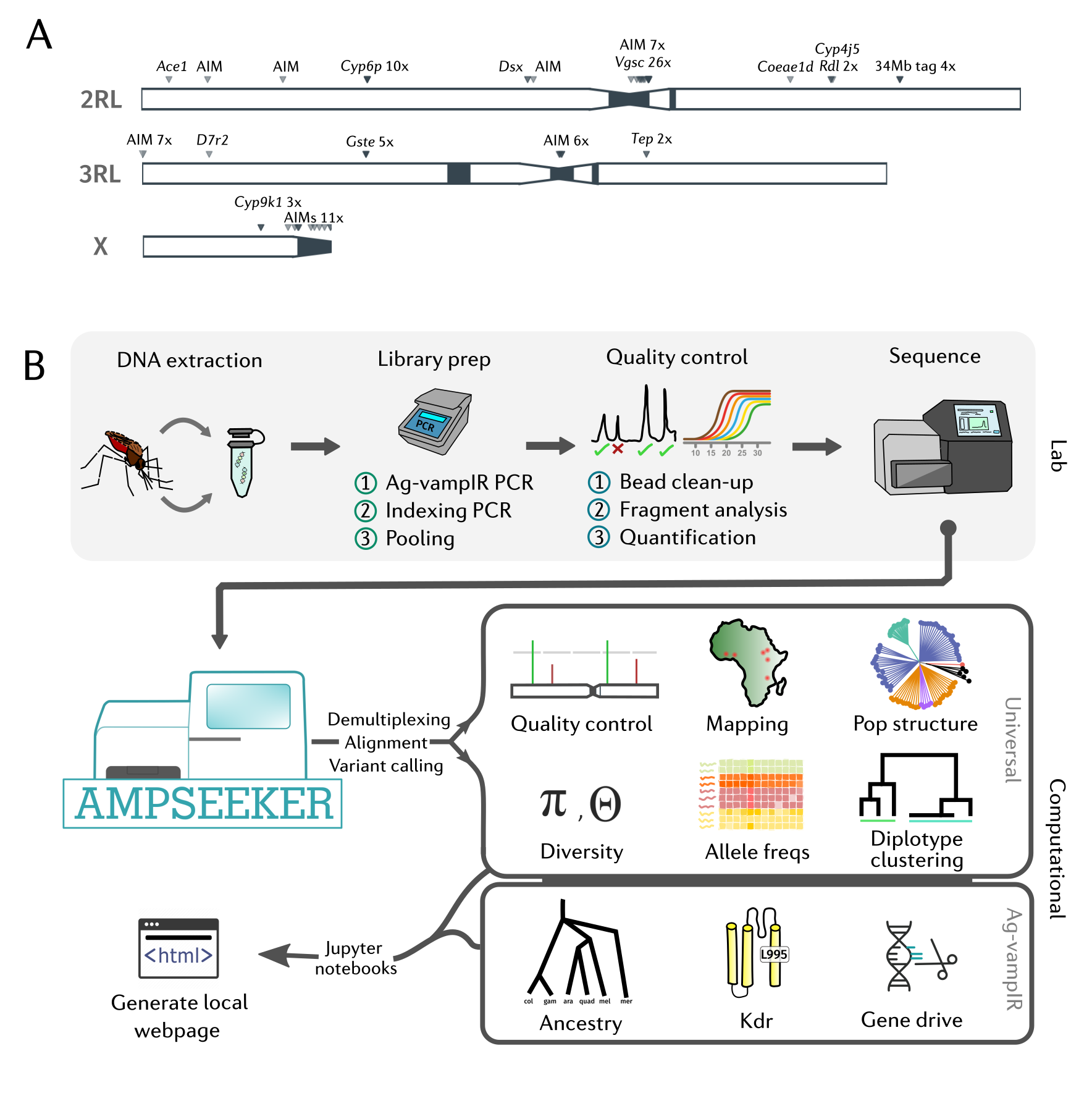
PCR1 (locus-specific). All the primer pairs go into one tube with the mosquito’s DNA, each at low concentration (10 uM stocks in the Ag-vampIR protocol). Every pair amplifies its own short target. This is the step that panel design has to make work: 80 pairs means 160 primers in one reaction, and every one of them can interact with every other.
PCR2 (indexing). The PCR1 product goes into a second reaction containing sample-specific index (barcode) sequences and the Illumina adapters, which are appended to the ends of every amplicon from that mosquito. Ag-vampIR uses 96 custom i7 indexes and 16 i5 indexes; because indexes are read in pairs, 96 x 16 gives a theoretical 1,536 samples per flow cell.
The locus-specific primers carry the adapter tails from the start, so PCR2 has something to prime on:
F: ACACTCTTTCCCTACACGACGCTCTTCCGATCT + locus-specific forward
R: TCGGCATTCCTGCTGAACCGCTCTTCCGATCT  + locus-specific reverse
Pool, clean, quantify, sequence. Plates are pooled, bead-cleaned, sized on a Tapestation or Bioanalyzer, quantified by qPCR, diluted and loaded. Ag-vampIR ran 542 samples on one Illumina MiSeq v2 kit (150 bp reads, about 5 Gb of output).
One design detail worth knowing, because it is invisible in any in-silico check: the Ag-vampIR primers have their second-to-last base replaced with a 2’-O-methyl base, a modification that suppresses primer dimer formation (after McKerrell et al. 2015). Chemistry can fix problems that primer selection alone cannot.
Coverage, and how much you need
With amplicon data, “coverage” means reads per amplicon per sample, and it is set by how you divide the run’s reads:
reads per amplicon per sample ~ total reads / (samples x amplicons)A MiSeq v2 kit gives roughly 15 million read pairs. Spread over 542 samples and 82 amplicons that is about 340 read pairs per amplicon per sample - far more than the 20-30x you need to call a diploid genotype confidently, which is the point: the margin absorbs the fact that amplification is never even. Some amplicons always run hot and some cold, some samples have degraded DNA, and the Ag-vampIR authors note that skipping DNA normalisation before PCR1 costs evenness between plates. Ag-vampIR’s own QC dropped 542 samples to 467 on depth, heterozygosity and PCA outliers.
Two consequences for design:
Uneven coverage is a design problem, not just a lab problem. An amplicon whose primers have a poor Tm match, or that competes badly in the multiplex, is the one that drops out - and a dropped amplicon is missing data at exactly the locus you cared about.
You can read copy number off depth. Since every amplicon in a sample is amplified from the same input DNA, relative depth carries information about copy number - which is how an amplicon panel can report on the Cyp6aa1 duplication without a separate qPCR, if the panel includes an amplicon inside the duplicated region and enough single-copy amplicons to normalise against.
Amplicon sequencing versus WGS versus qPCR
| qPCR / LNA assay | Amplicon sequencing | Whole-genome sequencing | |
|---|---|---|---|
| Cost per sample | ~$2.50 per locus | ~0.10 each) | >$100 |
| Loci per sample | 1-4 | 50-500 | all of them |
| Novel variants | no | only within the amplicons | yes |
| Copy number | one locus per assay | relative depth across amplicons | genome-wide, breakpoints |
| Species / ancestry | one marker at a time | AIM panel, hybrids detectable | full population genetics |
| Equipment in country | qPCR machine | MiSeq / MiniSeq | none, sent away |
| Turnaround | hours | days | weeks to months |
| Sample size feasible | hundreds | thousands | tens to hundreds |
The trade-off is fixed and worth stating plainly: an amplicon panel is biased towards what you already know. Resistance mechanisms arising outside the targeted regions will be missed, and Anopheles evolves new mechanisms readily. The healthy division of labour is WGS (or RNA-seq, as on Day 1) for discovery, and amplicon panels for surveillance of what discovery found - which is precisely the arc of this course.
The payoff of cheapness is statistical power. Because the Siaya samples were affordable to sequence in bulk, Ag-vampIR could do a genotype-phenotype association study on 252 phenotyped mosquitoes and find seven independent variants associated with surviving deltamethrin nets - an analysis that would have been prohibitive at WGS prices. You will re-run it in module 4.3.
Illumina or Nanopore?
Both are used for amplicon panels, and the choice is mostly about error profile and logistics.
| Illumina (MiSeq, MiniSeq, iSeq) | Oxford Nanopore (MinION, Flongle) | |
|---|---|---|
| Read length | 150-300 bp, so amplicons are kept short | kilobases, so long amplicons are fine |
| Raw error rate | very low, ~0.1%, mostly substitutions | higher, ~1-5%, indel-rich in homopolymers |
| SNP calling | straightforward at 20-30x | needs high depth and indel-aware tools |
| Capital cost | tens of thousands | hundreds to low thousands |
| Run logistics | fixed kit sizes, cold chain, batch to fill a run | run one plate today, stop when done |
| Barcoding | i5/i7 index pairs, 1,536 samples | native or PCR barcodes, typically fewer |
For SNP genotyping panels like Ag-vampIR, Illumina’s accuracy is the deciding factor, and the 200 bp amplicon length is chosen so 2 x 150 bp reads cover each amplicon end to end with overlap. Nanopore comes into its own where read length is the point - phasing a whole Vgsc haplotype in one read, spanning a CNV breakpoint, or resolving a transposon insertion like the ZZB element that no short amplicon can capture - and where a lab needs to run a handful of samples now rather than wait to fill a MiSeq kit.
2. What makes multiplex design hard
Designing one primer pair, as in module 4.1, means satisfying primer3 and checking Ag3 frequencies. Designing a pool means all of that, plus constraints that only exist between primers - and those grow quadratically. Eighty pairs is 160 primers and 12,720 pairwise combinations to check.
1. Primer dimers. Any two primers whose 3’ ends are complementary can prime each other.
The result is a short, efficiently amplified product that consumes reagents and reads, and
suppresses the real amplicons. This is the dominant failure mode of large multiplexes.
multiply scores every primer pair against every other with a Smith-Waterman-style alignment
weighted by nearest-neighbour thermodynamics and by proximity to the 3’ end, and treats the
worst interactions as a cost to minimise.
2. Tm matching. All amplicons share one cycling programme, so their annealing temperatures
must be compatible. A primer pair with Tm 55 will amplify inefficiently at an annealing
temperature chosen for pairs at Tm 62, and that amplicon drops out. This is why
PRIMER_PAIR_MAX_DIFF_TM matters much more in a panel than in a single assay, and why
Ag-vampIR used a wide but deliberately controlled window (min 50, opt 58, max 68 in the mprimer
run).
3. Off-target amplicons. In a pool, any forward primer can pair with any reverse primer, so
you must check not just whether a primer binds elsewhere but whether any two primers flank a
plausible product anywhere in the genome. multiply BLASTs every primer against the genome,
keeps hits that could support extension, and enumerates the resulting predicted amplicons.
Nearby targets in a cluster are the usual offenders: in the design we run below, forward primers
from the Cyp6p3 amplicon can pair with reverse primers from Cyp6p4 to give ~2.2 kb products,
because those targets are only 5 kb apart on 2R.
4. SNPs in primer sites. Exactly as in 4.1, but now a null allele is silent: instead of a
failed reaction you get one amplicon missing from one sample, which looks like missing data. In
a panel intended for several populations the primers must be clean in all of them. multiply
supports this through its snpcheck step, which counts variants from a population variation
track under each candidate primer and feeds the count into the cost function.
5. Amplicon length. Short enough for your read length (200 bp for 2 x 150 Illumina), long enough to leave primer3 room to find good primers, and similar between amplicons - length differences bias both PCR and bead clean-ups towards the short ones.
6. Tiling and spacing. Two targets closer together than the amplicon length cannot both have independent primers; you either merge them into one amplicon or accept overlapping designs. Ag-vampIR packs eight amplicons into the Cyp6p locus for this reason.
3. Case study: Ag-vampIR
Ag-vampIR (the An. gambiae Vector Amplicon Marker Panel for Insecticide Resistance) targets 90 SNP markers across 82 amplicons of about 200 bp each, on AgamP4, for Illumina. Primers were designed with an in-house modified version of MPprimer, except three amplicons (Vgsc-V402L, Vgsc-I1527T and doublesex) added later with AnoPrimer.
Let’s look at what it actually targets, straight from the panel’s BED file.
import pandas as pd

AGVAMPIR_BED = (
    "https://raw.githubusercontent.com/sanjaynagi/AmpSeeker/main/config/ag-vampir.bed"
)

panel = pd.read_csv(
    AGVAMPIR_BED,
    sep="\t",
    header=None,
    names=["contig", "start", "end", "amplicon", "target", "ref", "alt"],
)

print(f"{len(panel)} targets on {panel.amplicon.nunique()} amplicons\n")
panel.head()
def classify(target):
t = str(target)
if t.startswith("AIM"):
return "ancestry informative marker"
if t.startswith("Vgsc"):
return "Vgsc (target site, pyrethroids/DDT)"
if t.startswith("Rdl"):
return "Rdl (target site, cyclodienes)"
if t.startswith("Ace1"):
return "Ace1 (target site, OP/carbamate)"
if t.startswith("Cyp6"):
return "Cyp6aa/p cluster (metabolic)"
if t.startswith("Cyp9k1"):
return "Cyp9k1 (metabolic)"
if t.startswith("Cyp4j5"):
return "Cyp4j5 / 2La karyotype"
if t.startswith("Gste"):
return "Gste cluster (metabolic)"
if t.startswith("34mb"):
return "34 Mb sweep (2L)"
if t.startswith("Coeae"):
return "carboxylesterase (metabolic)"
if t.startswith("Tep1"):
return "Tep1 (Plasmodium refractoriness)"
if t.startswith("DSX"):
return "doublesex (gene drive target)"
if t.startswith("D7"):
return "D7 salivary protein"
return "other"
panel["class"] = panel.target.apply(classify)
summary = (
panel.groupby("class")
.agg(n_targets=("target", "size"), n_amplicons=("amplicon", "nunique"))
.sort_values("n_targets", ascending=False)
)
summaryRead that table as a set of design decisions:
35 ancestry informative markers (AIMs) spread over all five chromosome arms. These were chosen to separate An. gambiae from An. coluzzii, but in practice they resolved An. arabiensis and An. melas as well (F1 > 0.99 with a classifier trained on 7,363 whole-genome-sequenced Ag3 individuals). Spreading them across arms is what lets the panel see mosaic ancestry: the Siaya colony turned out to look like An. gambiae on chromosome 2 and the X but An. coluzzii-like on chromosome 3.
A dense tile over Vgsc - 26 targets across the gene - because kdr is not one mutation but a set of haplotypes. Tiling the locus lets you read secondary mutations (T791M, N1570Y, A1746S, P1874S/L) and so tell 995F haplotype backgrounds apart: Obuasi and VK7 share the F1 background, while Siaya carries F2.
Tagging SNPs at swept loci (
Cyp6_tag*,Gste_tag*,Cyp9k1_tag*,34mb_tag*). These are not necessarily causal. They mark a swept haplotype identified in Ag1000G, which is cheaper and more robust than trying to genotype an unknown causal variant. This is the direct link back to your Day 3 selection-atlas work: a sweep you find in the atlas can be turned into a tagging-SNP amplicon.Target-site mutations with known mechanisms: Ace1-G280S, Rdl-A296S/G, Vgsc codons.
Two amplicons at the doublesex intron 4-exon 5 boundary, the target of the population suppression gene drive - included so that the panel can monitor the drive target site for resistance alleles.
Now find the markers for the triple mutant and the loci that mattered in Siaya.
triple_mutant = ["Cyp6p4_I236M", "Cyp6p3_I88T"]
panel[panel.target.isin(triple_mutant) | panel.target.str.startswith("Cyp6_tag")]
Eight amplicons cover the Cyp6aa/p locus. In the Siaya association study (module 4.3) thirteen SNPs in this cluster - including Cyp6p4-I236M itself, at an odds ratio of about 3.4 - were associated with surviving PermaNet 2.0 deltamethrin nets, together with fourteen SNPs at the 34 Mb sweep and four at Cyp4j5. The Gste and Cyp9k1 tags, by contrast, were monomorphic or absent in Siaya and told us nothing there - a reminder that a panel designed for a continent will always carry markers that are uninformative in any one place, and that this is the right trade-off for a shared panel.
Notice also what the panel cannot do. There is no marker for the ZZB transposable element
insertion, the third component of the triple mutant, because a short amplicon designed on the
reference genome cannot detect an insertion absent from that reference. And Cyp6aa1 copy
number is read from amplicon depth rather than from any single marker.
4. Case study: ANOSPP (lecture only)
ANOSPP solves a different problem: which species is this mosquito, anywhere in the genus, and is it carrying Plasmodium?
Design. 62 phylogenetically informative nuclear loci of about 160 bp, chosen to amplify across a “generic” Anopheles genome rather than in one species, plus two conserved Plasmodium mitochondrial loci. Two-step multiplex PCR with barcoding, roughly 800 mosquitoes per MiSeq run. Non-destructive extraction leaves the specimen available for morphological checks.
Why the design differs from Ag-vampIR. Ag-vampIR targets known positions in one reference genome, so its primers can sit on fixed sequence and its analysis is genotype calling. ANOSPP must work across a genus whose members are tens of millions of years divergent, so its primers sit in conserved sequence flanking variable regions, and its analysis compares haplotypes rather than calling reference-based genotypes. That is why the anospp-analysis pipeline starts from DADA2 haplotype tables and classifies samples by k-mer distance to a reference index (
anospp-prep,anospp-qc,anospp-plasm,anospp-nn,anospp-vae,anospp-agg), with a dedicated step for the An. gambiae complex.Scale. The project aims at 500,000 mosquitoes across Africa, and needs at least ten expertly identified individuals per species to build out the reference index - a reminder that a panel of this kind is only as good as its reference data.
The two panels are complementary: ANOSPP tells you what you caught, Ag-vampIR tells you what resistance it carries. Neither replaces the other, and a survey often runs both.
5. Practical: design a multiplex with multiply
multiply is an open-source command-line tool for designing multiplex PCRs, written by Jason A. Hendry (de Cesare et al. 2024, Nat Commun Cesare et al. (2023)). It is not our software, and it was written with Plasmodium in mind, but its genome registry includes An. gambiae (AgamP4) and the design logic is general.
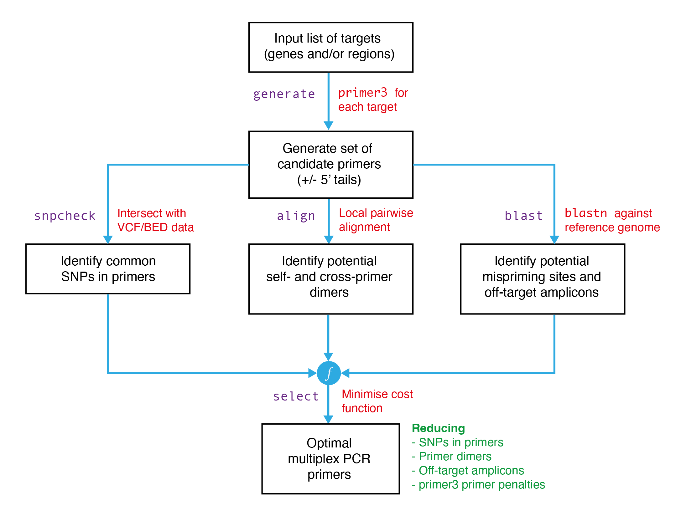
Six steps, matching the constraints in section 2:
| Command | What it does |
|---|---|
multiply download | fetch the reference FASTA and GFF for your organism |
multiply generate | run primer3 over every target, with several settings files, to build a pool of candidate pairs |
multiply view | plot candidate primer locations against the annotation |
multiply snpcheck | count known variants under each candidate primer |
multiply align | score every primer against every other for dimer potential |
multiply blast | BLAST all primers, predict on- and off-target amplicons |
multiply select | combine the above into a cost function and search for the best multiplex |
multiply pipeline | run all of the above in order |
The key idea is the last step. Each candidate primer carries individual costs (its primer3
penalty, its number of predicted mispriming sites, its SNP load) and each pair of primers
carries a pairwise cost (dimer potential). Choosing one primer pair per target is then a
combinatorial optimisation problem, which multiply select attacks greedily and benchmarks
against random search.
Installing it
multiply needs three conda-installed binaries - primer3_core, bedtools and blastn - so
pip install alone is not enough. Two routes:
Route A: Colab with condacolab. Workable, but note two things. condacolab.install()
restarts the kernel, so it must be the only statement in its cell and you re-run the
imports afterwards; and the whole setup takes 5-10 minutes.
Route B: the course Codespace (recommended). The devcontainer already has conda, so you skip the restart dance and keep the environment between sessions. This is also where you will run Snakemake workflows on Days 1 and 4.
Either way, pin the Python stack. We verified the pins below on both osx-arm64 and
linux-64; with a current pandas (>= 2.0) the blast and view steps of multiply crash,
because the code predates the removal of some deprecated pandas behaviour.
# environment.yml
name: multiply
channels: [conda-forge, bioconda]
dependencies:
  - python=3.10
  - primer3=2.6.1
  - bedtools=2.31.1
  - blast=2.16.0
  - click=8.1
  - pandas=1.5.3
  - numpy=1.23.5
  - scipy=1.10
  - pysam=0.22
  - seaborn=0.12.2
  - matplotlib=3.7
  - numba=0.57
  - pip
If the install below fails or times out, skip to the next section: the design outputs are described in full, and you can read the practical without running it.
# Route A: Colab only. This cell RESTARTS THE KERNEL - that is expected.
# Skip it entirely in the Codespace.
import sys

IN_COLAB = "google.colab" in sys.modules

if IN_COLAB:
    !pip install -q condacolab
    import condacolab

    condacolab.install()
# after the restart (Colab), or as the first cell (Codespace)
import os
import subprocess
import sys
IN_COLAB = "google.colab" in sys.modules
PKGS = [
"primer3=2.6.1",
"bedtools=2.31.1",
"blast=2.16.0",
"click=8.1",
"pandas=1.5.3",
"numpy=1.23.5",
"scipy=1.10",
"pysam=0.22",
"seaborn=0.12.2",
"matplotlib=3.7",
"numba=0.57",
]
solver = "mamba" if IN_COLAB else "conda"
print(f"installing with {solver}; this takes several minutes")
!{solver} install -y -q -c conda-forge -c bioconda {" ".join(PKGS)}import os
# clone into /content on Colab, or the working directory in the Codespace
MULTIPLY_DIR = "/content/multiply" if os.path.isdir("/content") else "./multiply"
if not os.path.isdir(MULTIPLY_DIR):
!git clone -q https://github.com/JasonAHendry/multiply {MULTIPLY_DIR}
!pip install -q --no-deps -e {MULTIPLY_DIR}
!cd {MULTIPLY_DIR} && multiply --helpmultiply resolves its settings, genome registry and results directories relative to the
repository root, so every command below is run from inside MULTIPLY_DIR.
Now fetch the An. gambiae AgamP4 reference. This is about 250 MB of FASTA plus a GFF, which
multiply converts to a CSV of gene positions; allow a few minutes.
!cd {MULTIPLY_DIR} && multiply download --available!cd {MULTIPLY_DIR} && multiply download -g AnophelesGambiaeThe design file
A multiply design is an .ini file. Targets can be genes (by identifier, from the GFF) or
regions (a BED file with a name in column 4). We use regions, because our targets are SNPs
rather than whole genes - a whole Cyp6aa1 gene target would ask for a 2 kb amplicon.
The course repository holds a ready-made design for the class panel, covering the Busia sweep loci, the triple-mutant markers, and the Siaya-informative loci from module 4.3.
REPO = "sanjaynagi/anopheles-omics-training"
BASE = f"https://raw.githubusercontent.com/{REPO}/main/day-4/multiply"

!wget -q -O {MULTIPLY_DIR}/designs/busia-panel.ini {BASE}/busia-panel.ini
!mkdir -p {MULTIPLY_DIR}/designs/beds
!wget -q -O {MULTIPLY_DIR}/designs/beds/busia-panel.bed {BASE}/busia-panel.bed

print(open(f"{MULTIPLY_DIR}/designs/busia-panel.ini").read())print(open(f"{MULTIPLY_DIR}/designs/beds/busia-panel.bed").read())Three choices in that design file are worth pausing on.
min_size_bp = 150,max_size_bp = 250. Short amplicons, so 2 x 150 bp reads cover each one end to end.multiplypads each target bymax_size_bp / 2either side to give primer3 somewhere to search, and refuses a design where those pads overlap - which is the mechanical reason closely spaced targets have to be merged.primer3_settings = default, stringent, relaxed. primer3 is run once per settings file per target and the results pooled, so the candidate pool contains both conservative and permissive options. More settings means a larger pool and a better chance that the optimiser can avoid dimers.include_tails = False. The Illumina adapter tails are added after design, not during. With tails on,multiply’s BLAST step cannot match its hits back to the recorded primer positions, so it finds no on-target amplicons and the pipeline fails. Design the locus-specific primers first, then prepend the adapters to the ordering table.
Adapt the BED file to your own loci by editing it: one line per target, contig, 0-based start,
end, name.
Run the pipeline
!cd {MULTIPLY_DIR} && multiply pipeline -d designs/busia-panel.iniOn ten targets this takes well under a minute after the genome download (the BLAST database is
built once, on first use). Expect a FutureWarning from the BLAST annotator, and possibly a
multiply view warning for targets with no nearby annotation - neither is fatal.
Walk through the output as it goes past:
multiply generatereports candidate pairs per target - typically 5-8 unique pairs from 15 primer3 runs, the duplicates being the same pair found by several settings files. A target with zero pairs stops the pipeline; relax the amplicon range or the primer3 settings.multiply snpcheckwill say “No variation data is available for AnophelesGambiae”. This is expected:multiplyships variation tracks for P. falciparum only, so for An. gambiae this cost term is simply absent andselectruns without it. That is the one real gap in this workflow for our purposes - see Exercise 2.multiply alignwrites every primer-primer alignment, worst first, as an ASCII diagram.multiply blastreports BLAST hits, putative binding sites and predicted off-target amplicons.multiply selectprints the cost of the greedy solution against a random-search benchmark (lower is better) and writes the chosen multiplexes.
RESULTS = !ls -d {MULTIPLY_DIR}/results/*busia-panel
RESULTS = RESULTS[0]
!ls {RESULTS} {RESULTS}/select
candidates = pd.read_csv(f"{RESULTS}/table.candidate_primers.csv")
print(f"{len(candidates)} candidate primers")
candidates.groupby("target_name").pair_name.nunique().rename("n_candidate_pairs")chosen = pd.read_csv(f"{RESULTS}/select/table.multiplexes_information.csv")
cols = ["target_name", "primer_name", "direction", "seq", "length", "tm", "gc", "product_bp"]
chosen.query("in_multiplex00 == True")[cols]That is your panel: one primer pair per target, chosen to minimise the combined cost. Check the
tm column spread - if it is wider than about 3 degrees C, tighten primer3_settings to
stringent alone and re-run, because the widest-spread amplicons are the ones that will drop
out.
multiply writes three alternative multiplexes (multiplex00, 01, 02) so you have
fallbacks, and an ordering table ready to paste into a synthesis order.
order = pd.read_csv(f"{RESULTS}/select/table.multiplexes_order.csv")
order.head(8)
Reading the dimer output
The worst interactions in the pool, worst first. Each diagram shows two primers annealed to each
other, with | for a matched base pair; the score is more negative the more stable the dimer.
What matters is not the raw score but where the complementarity sits: pairing at the 3’ ends
is what lets a polymerase extend and turn a transient duplex into a real product.
print(open(f"{RESULTS}/align/alignment_diagrams.txt").read()[:2000])dimers = pd.read_csv(f"{RESULTS}/align/table.alignment_scores.csv")
dimers.head(10)Note that many of the worst interactions are between candidate primers for the same target,
which can never be in the same multiplex - so read this table alongside the chosen multiplex.
multiply select writes the interactions for the primers it actually chose to
select/multiplex00/diagrams.multiplex00.primer_interactions.txt and plots them as a heatmap;
that is the file to inspect before ordering.
print(
    open(f"{RESULTS}/select/multiplex00/diagrams.multiplex00.primer_interactions.txt").read()[
        :1200
    ]
)
Reading the off-target output
offtarget = pd.read_csv(f"{RESULTS}/blast/table.offtarget_amplicons.csv", index_col=0)
print(f"{len(offtarget)} predicted off-target amplicons")
offtarget.head(10)
mispriming = pd.read_csv(f"{RESULTS}/blast/table.blast.candidate_primers.summary.csv")
mispriming.sort_values("predicted_bound", ascending=False).head(10)Two things to take from these tables.
The off-target amplicons are dominated by cross-pairings within the Cyp6 cluster: a forward primer from the Cyp6p3 amplicon with a reverse primer from Cyp6p4 gives a product of about 2.2 kb, because those targets sit 5 kb apart on 2R. Long products like these amplify poorly under a short-amplicon cycling programme, so they are a nuisance rather than a disaster - but they are exactly what you would fail to notice designing each assay separately, and they are why clustered targets need checking as a pool.
predicted_boundcounts plausible binding sites per primer. High values flag primers sitting in repetitive sequence; you can see the same phenomenon in the X-linked Cyp9k1 candidates, which return far more BLAST hits than the autosomal ones.
Exercise 1
Add one of your own candidate loci to the panel and re-run the design.
Pick a SNP from your Day 3 work (or a position inside one of your candidate genes), add a line to the BED file, and re-run the pipeline. Then answer: did primer3 find candidate pairs for your target; is your chosen pair’s Tm within 3 degrees C of the rest of the panel; and does your target introduce any new off-target amplicons?
Show answer
bed_path = f"{MULTIPLY_DIR}/designs/beds/busia-panel.bed"

# a SNP at contig:position (1-based), written as a 0-based BED interval with 10 bp of context
contig, pos, name = "2L", 2422651, "my_target"
with open(bed_path, "a") as bed:
    bed.write(f"{contig}\t{pos - 1 - 10}\t{pos + 10}\t{name}\n")

!cd {MULTIPLY_DIR} && multiply pipeline -d designs/busia-panel.ini
multiply refuses to overwrite an existing results directory for the same design on the same day, so either delete it first or change name in the [Output] section.
Things that plausibly go wrong, all of them informative:
No primer pairs for your target. The commonest cause is repetitive or AT-rich flanking sequence. Widen
max_size_bp, or addvariabletoprimer3_settings.Pads overlap with a neighbouring target. Your locus is within
max_size_bp / 2of another; merge the two into a single amplicon covering both SNPs.A wide Tm spread after adding your target. Re-run with
primer3_settings = stringentso every candidate is drawn from the tight-Tm settings file.
# your answer hereExercise 2
multiply snpcheck found no variation data for An. gambiae, so the panel above was chosen
without considering SNPs in primer binding sites - the very thing module 4.1 spent its time
on.
Using what you know from 4.1, check the chosen primers yourself against the Busia cohort, and
say which (if any) you would replace. Then suggest how you would supply multiply with a
variation track so that snpcheck could do this for you.
Show answer
%pip install -q --no-warn-conflicts anoprimer==2.0.8 malariagen_data==15.9.0
import AnoPrimer

BUSIA_SAMPLE_SETS = "1178-VO-UG-LAWNICZAK-VMF00025"
BUSIA_QUERY = "cohort_admin2_quarter == 'UG-E_Busia_gamb_2016_Q2'"

for _, row in chosen.query("in_multiplex00 == True").iterrows():
    print(row.primer_name)
    AnoPrimer.check_my_oligo(
        sequence=row.seq,
        sample_sets=BUSIA_SAMPLE_SETS,
        sample_query=BUSIA_QUERY,
    )
check_my_oligo BLATs each sequence and plots Ag3 frequencies across it, so you can apply the 4.1 rules: reject anything segregating in the 3’-most five bases, or at high frequency anywhere in the primer. Note it is slow (one BLAT plus one Ag3 query per primer) and that BLAT sometimes returns no hit for a 20-mer.
To do it properly inside multiply, its snpcheck step intersects a primer BED with variation files listed in genomes/variation/<Genome>/files.json. So you would write one BED of Ag3 segregating sites per cohort - for example everything above 2% minor allele frequency in Ugandan An. gambiae, obtained from ag3.snp_allele_frequencies() - register it in that JSON, and add a matching cost term in settings/select/individual_costs.ini pointing at the new column. The primer-level SNP count then becomes part of the optimisation rather than an afterthought. This is precisely the gap AnoPrimer was written to fill for single assays.
# your answer hereExercise 3
Your panel has ten amplicons. Ag-vampIR has 82, and ANOSPP 64.
Suppose you wanted to grow yours to 80 amplicons for a national programme. Which of the six design constraints in section 2 gets disproportionately harder, and what would you change about the workflow above?
Show answer
Dimers, because the number of primer-primer interactions grows quadratically: 10 amplicons means 20 primers and 190 pairwise comparisons, while 80 amplicons means 160 primers and 12,720. Tm matching and amplicon length scale linearly and stay manageable; off-target checking grows quadratically too, but off-target products are usually tolerable whereas a strong dimer can suppress the whole reaction.
Practical changes:
Make the candidate pool bigger, not smaller, so the optimiser has room to avoid dimers - more
primer3_settingsfiles, a wider amplicon range.Rely on the optimiser rather than on eyeballing. At 12,720 interactions you cannot inspect diagrams; you set cost weights and compare the greedy result with the random benchmark.
Expect to split the panel into pools, and to iterate: design, test in the lab, drop the amplicons that fail, redesign them. Ag-vampIR is the product of that loop, not of one successful run.
Use chemistry as well as sequence. Ag-vampIR’s 2’-O-methyl substitution at the penultimate base suppresses dimers no in-silico step can remove.
Budget the reads. 80 amplicons x 1,536 samples on one flow cell is a real constraint on depth; adding amplicons costs coverage per amplicon unless you reduce samples per run.
# your answer hereQuiz
%pip install -q jupyterquiz==2.9.6.4
from jupyterquiz import display_quiz

display_quiz(
    "https://raw.githubusercontent.com/sanjaynagi/anopheles-omics-training/main/quizzes/4-2-amplicon-panel-design.json"
)Summary
Targeted amplicon sequencing multiplexes 50-500 short PCR products per sample, adds sample-specific i5/i7 indexes in a second PCR, and pools over a thousand samples on one run. Ag-vampIR costs about **2.50 per locus by LNA qPCR and over $100 per sample by WGS.
Coverage is total reads divided by (samples x amplicons), and the margin over the 20-30x needed for genotype calling exists to absorb uneven amplification. Relative depth across amplicons also carries copy-number information.
Illumina suits SNP panels (low error, short amplicons of about 200 bp); Nanopore suits long amplicons, haplotype phasing, insertions and small, flexible batches.
Multiplex design adds constraints that exist only between primers - dimers above all, since they grow quadratically - plus Tm matching, cross-paired off-target amplicons, SNPs in primer sites, amplicon length and target spacing.
Ag-vampIR targets 90 SNPs on 82 amplicons: 35 AIMs across all arms, a dense Vgsc tile, target-site mutations (Ace1, Rdl), tagging SNPs for the Cyp6aa/p, Gste, Cyp9k1 and 34 Mb sweeps, Cyp4j5, Tep1 and doublesex. A sweep found in the selection atlas becomes a tagging-SNP amplicon.
ANOSPP targets 62 conserved-flank loci across the genus plus two Plasmodium mitochondrial loci, and is analysed as haplotypes rather than reference genotypes - a different problem needing a different design.
multiply turns panel design into an optimisation: candidate primers from primer3, costed by primer3 penalty, mispriming and SNP load, with dimer potential as a pairwise cost, then a greedy search for the best set. Its An. gambiae SNP track is missing, so combine it with AnoPrimer’s Ag3 checks.
Record the assay you would use for each marker in your gene dossier - and whether you would run it as a qPCR assay or ask for it to be added to a panel.
Well done!
You have designed a small multiplex panel for the loci this course discovered, and you know why the two real panels in this field look the way they do. In module 4.3 you analyse real Ag-vampIR data from Siaya with AmpSeeker, and test whether these markers predict which mosquitoes survive a deltamethrin net.
References
Nagi SC et al. (2025) Targeted genomic surveillance of insecticide resistance in African malaria vectors. bioRxiv. SRA PRJNA1207724.
de Cesare M, Mwenda M, Jeffreys AE et al. (2024) Flexible and cost-effective genomic surveillance of P. falciparum malaria with targeted nanopore sequencing. Nature Communications 15:1413. Cesare et al. (2024) (introduces multiply; J. A. Hendry is senior author)
Makunin A et al. (2022) A targeted amplicon sequencing panel to simultaneously identify mosquito species and Plasmodium presence across the entire Anopheles genus. Molecular Ecology Resources 22(1):28-44. Makunin et al. (2021)
Njoroge H et al. (2022) Identification of a rapidly spreading triple mutant for high-level metabolic insecticide resistance in Anopheles gambiae provides a real-time molecular diagnostic for antimalarial intervention deployment. Molecular Ecology 31(16):4307-4318. Njoroge et al. (2022)
Shen Z et al. (2010) MPprimer: a program for reliable multiplex PCR primer design. BMC Bioinformatics 11:143. Shen et al. (2010)
Jacob CG et al. (2021) Genetic surveillance in the Greater Mekong subregion and South Asia to support malaria control and elimination. eLife 10:e62997. Jacob et al. (2021)
McKerrell T et al. (2015) Leukemia-associated somatic mutations drive distinct patterns of age-related clonal hemopoiesis. Cell Reports 10(8):1239-1245. McKerrell et al. (2015)
Johnston AD, Lu J, Ru K, Korbie D, Trau M (2019) PrimerROC: accurate condition-independent dimer prediction using ROC analysis. Scientific Reports 9:209. Johnston et al. (2019)
Lucas ER et al. (2019) A high-throughput multi-locus insecticide resistance marker panel for tracking resistance emergence and spread in Anopheles gambiae. Scientific Reports 9:13335. https://
doi .org /10 .1038 /s41598 -019 -49892-6 Miles A et al. (2017) Genetic diversity of the African malaria vector Anopheles gambiae. Nature 552:96-100. Springer Science,Business Media LLC (2017)
- Shen, Z., Qu, W., Wang, W., Lu, Y., Wu, Y., Li, Z., Hang, X., Wang, X., Zhao, D., & Zhang, C. (2010). MPprimer: a program for reliable multiplex PCR primer design. BMC Bioinformatics, 11(1). 10.1186/1471-2105-11-143
- de Cesare, M., Mwenda, M., Jeffreys, A. E., Chirwa, J., Drakeley, C., Schneider, K., Ghinai, I., Busby, G. B., Hamainza, B., Hawela, M., Bridges, D. J., & Hendry, J. A. (2023). Flexible and cost-effective genomic surveillance of P. falciparum malaria with targeted nanopore sequencing. 10.1101/2023.02.06.527333
- de Cesare, M., Mwenda, M., Jeffreys, A. E., Chirwa, J., Drakeley, C., Schneider, K., Mambwe, B., Glanz, K., Ntalla, C., Carrasquilla, M., Portugal, S., Verity, R. J., Bailey, J. A., Ghinai, I., Busby, G. B., Hamainza, B., Hawela, M., Bridges, D. J., & Hendry, J. A. (2024). Flexible and cost-effective genomic surveillance of P. falciparum malaria with targeted nanopore sequencing. Nature Communications, 15(1). 10.1038/s41467-024-45688-z
- Makunin, A., Korlević, P., Park, N., Goodwin, S., Waterhouse, R. M., von Wyschetzki, K., Jacob, C. G., Davies, R., Kwiatkowski, D., St. Laurent, B., Ayala, D., & Lawniczak, M. K. N. (2021). A targeted amplicon sequencing panel to simultaneously identify mosquito species and Plasmodium presence across the entire Anopheles genus. Molecular Ecology Resources, 22(1), 28–44. 10.1111/1755-0998.13436
- Njoroge, H., van’t Hof, A., Oruni, A., Pipini, D., Nagi, S. C., Lynd, A., Lucas, E. R., Tomlinson, S., Grau‐Bove, X., McDermott, D., Wat’senga, F. T., Manzambi, E. Z., Agossa, F. R., Mokuba, A., Irish, S., Kabula, B., Mbogo, C., Bargul, J., Paine, M. J. I., … Donnelly, M. J. (2022). Identification of a rapidly‐spreading triple mutant for high‐level metabolic insecticide resistance in Anopheles gambiae provides a real‐time molecular diagnostic for antimalarial intervention deployment. Molecular Ecology, 31(16), 4307–4318. 10.1111/mec.16591
- Jacob, C. G., Thuy-Nhien, N., Mayxay, M., Maude, R. J., Quang, H. H., Hongvanthong, B., Vanisaveth, V., Ngo Duc, T., Rekol, H., van der Pluijm, R., von Seidlein, L., Fairhurst, R., Nosten, F., Hossain, M. A., Park, N., Goodwin, S., Ringwald, P., Chindavongsa, K., Newton, P., … Miotto, O. (2021). Genetic surveillance in the Greater Mekong subregion and South Asia to support malaria control and elimination. eLife, 10. 10.7554/elife.62997
- McKerrell, T., Park, N., Moreno, T., Grove, C. S., Ponstingl, H., Stephens, J., Crawley, C., Craig, J., Scott, M. A., Hodkinson, C., Baxter, J., Rad, R., Forsyth, D. R., Quail, M. A., Zeggini, E., Ouwehand, W., Varela, I., & Vassiliou, G. S. (2015). Leukemia-Associated Somatic Mutations Drive Distinct Patterns of Age-Related Clonal Hemopoiesis. Cell Reports, 10(8), 1239–1245. 10.1016/j.celrep.2015.02.005
- Johnston, A. D., Lu, J., Ru, K., Korbie, D., & Trau, M. (2019). PrimerROC: accurate condition-independent dimer prediction using ROC analysis. Scientific Reports, 9(1). 10.1038/s41598-018-36612-9
- (2017). Nature, 552(7683), 96–100. 10.1038/nature24995