
4.3 Analysing amplicon sequencing data with AmpSeeker
Theme: Tools & technology | Analysis
In Module 4.2 we saw how a multiplex amplicon panel is designed. Here we analyse data from one: Ag-vampIR, a panel of 82 amplicons that genotypes 90 SNPs in An. gambiae s.l., including insecticide resistance mutations, SNPs that tag known selective sweeps, and ancestry informative markers (AIMs) [1]. We analyse it with AmpSeeker, a Snakemake workflow that goes from reads to genotypes, quality control and an interactive results book [1].
The data come from a colony established in 2023 from Siaya, western Kenya, about 50 km from Busia. Mosquitoes were exposed to deltamethrin nets (PermaNet 2.0) in extended WHO cone tests and scored dead or alive. We also run the VK7 colony (An. coluzzii, Burkina Faso), sequenced on the same MiSeq run.
This is where the course storyline closes. On Days 1–3 we found genes overexpressed in the Busia colony and selective sweeps in the Busia 2016 atlas cohort at the Cyp6aa/p cluster (2R), 2L ~34 Mb, the Gste cluster (3R) and Cyp9k1 (X). Ag-vampIR has markers at all four loci. So: do the loci we found with RNA-seq and selection scans predict which mosquitoes survive? We follow our worked example, CYP6AA1, which sits in the 2R sweep, to the end.
Learning objectives
At the end of this module you will be able to:
Explain how amplicon sequencing data are processed: demultiplexing, trimming, alignment to a reference genome, and variant calling at targets.
Judge the quality of an amplicon run from coverage, sample and target failure, heterozygosity and negative controls.
Configure and run AmpSeeker from FASTQ files in a GitHub Codespace, and find your way around its results book.
Load AmpSeeker genotypes in Python and test markers for association with a phenotype using a binomial GLM with false discovery rate control.
Judge whether the Busia RNA-seq and selection results are supported by survival data from Siaya.
Setup
Colab already has pandas, plotly and statsmodels. We add scikit-allel to read VCF files.
%pip install -q --no-warn-conflicts scikit-allel==1.3.13import os
import tarfile
import urllib.request
import allel
import numpy as np
import pandas as pd
import plotly.express as px
import statsmodels.api as sm
from statsmodels.stats.multitest import fdrcorrection
import plotly.io as pio
pio.templates.default = "simple_white" # course style for every Plotly figure
AMPSEEKER_VERSION = "v0.7.0" # the release we pin for the course
COURSE_RAW = "https://raw.githubusercontent.com/sanjaynagi/anopheles-omics-training/main"
# TODO(data): AmpSeeker v0.7.0 run on all Siaya + VK7 samples: the config/ and results/ files listed
# in workflows/ampseeker/README.md, packed as ampseeker-siaya-vk7-results.tar.gz and uploaded to Zenodo.
RESULTS_URL = "https://zenodo.org/records/TODO/files/ampseeker-siaya-vk7-results.tar.gz"
# The AmpSeeker folder to read results from. In your codespace, after your own run has finished,
# you can set this to "/workspaces/AmpSeeker" to analyse your own results instead.
AMPSEEKER_DIR = "ampseeker-siaya-vk7"
DATASET = "siaya-vk7" # the `dataset` value in the config file; AmpSeeker uses it to name the VCFs# Replace with the genes you were assigned on Day 2 (see data/candidate-genes.tsv)
CANDIDATE_GENES = ["AGAP002862", "AGAP009193"] # CYP6AA1, GSTE4From reads to genotypes: how amplicon data are analysed
Whole-genome sequencing spreads reads over the whole genome at ~30× coverage. Amplicon sequencing does the opposite: a multiplex PCR copies a few dozen short regions (~200 bp each), and hundreds of mosquitoes are sequenced together on one run. Each target ends up with hundreds or thousands of reads, at a cost of around US$10 per sample for Ag-vampIR [1]. Because every read starts and ends at a primer, the analysis has its own steps and its own failure modes.
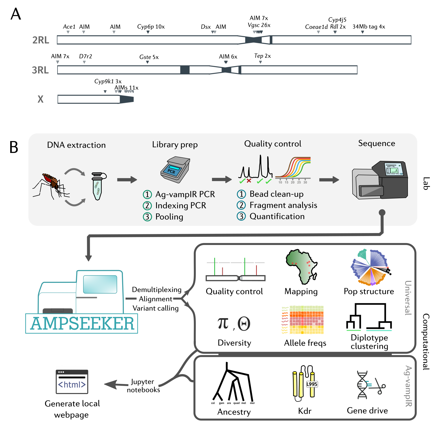
1. Demultiplexing. In the second PCR each sample gets a unique pair of index sequences (Ag-vampIR
uses 96 i7 × 16 i5 indexes, so up to 1,536 samples per run). The sequencer reads the indexes
separately, and demultiplexing (bcl-convert) sorts reads into one pair of FASTQ files per sample
using a SampleSheet.csv. A small fraction of reads always get the wrong sample, through index
misassignment on the flow cell or cross-contamination in the lab. AmpSeeker can start from the raw
MiSeq output folder (from-bcl: True) or, as today, from FASTQs that are already demultiplexed
(from-bcl: False); the SRA stores demultiplexed reads.
2. Trimming. fastp removes adapters and low-quality ends. With ~200 bp amplicons and
2 × 150 bp reads, the two reads of a pair overlap, and short products (primer dimers) read into the
adapter.
3. Alignment to the genome. Reads are aligned with bwa mem to the whole AgamP4 reference, not
just to the amplicon sequences. That way positions are in genome coordinates, the same as Ag3 and
the selection atlas, and reads from off-target products map elsewhere instead of being forced onto a
target.
4. Variant calling. bcftools mpileup and bcftools call genotype each sample, in two ways:
targets: only the panel’s SNPs, listed in
config/ag-vampir.bed. A genotype is reported even when the sample carries the reference allele, so “not called” means “no data”.amplicons: every position covered by reads, which finds SNPs the panel was not designed for.
Calls are annotated with snpEff (gene, amino acid change). Be careful with any SNP under a primer:
the primer sequence is copied into every read, so the read shows the primer’s base, not the
mosquito’s. A SNP in a primer site can also stop one allele from amplifying (allele dropout),
which makes heterozygotes look homozygous.
5. Quality control. Amplicons amplify with different efficiency, so coverage is never even. Look for:
Sample failure: low total coverage (poor DNA, failed PCR) and many missing calls.
Target failure: an amplicon with low coverage in every sample (a poor primer, primer dimers, or a SNP under a primer in this population).
Contamination: a sample containing DNA from two mosquitoes has too many heterozygous calls. AmpSeeker removes samples with outlying heterozygosity or outlying PCA positions within their cohort.
Negative controls (no-template wells): they should have almost no reads. Reads in a negative control measure background contamination and index misassignment for the whole plate. AmpSeeker drops samples whose names contain
Negativeordil(dilution replicates) from the analysis.
A first QC check, before running anything
The number of reads per sample is public in the ENA metadata. Let us compare the negative controls with real samples.
ena_url = (
    "https://www.ebi.ac.uk/ena/portal/api/filereport?accession=PRJNA1207724"
    "&result=read_run&fields=run_accession,sample_alias,read_count&format=tsv"
)
ena = pd.read_csv(ena_url, sep="\t")

# Our sample sheet for the Siaya + VK7 subset (built from the paper's metadata and ENA)
course_metadata = pd.read_csv(f"{COURSE_RAW}/workflows/ampseeker/metadata.tsv", sep="\t")
reads = course_metadata.merge(ena[["run_accession", "read_count"]], on="run_accession")

print(reads.groupby("cohort").read_count.describe()[["count", "min", "50%", "max"]])

fig = px.strip(
    reads, x="cohort", y="read_count", color="location", log_y=True,
    hover_data=["sample_id"], template="simple_white", height=400,
    title="Read pairs per sample (ENA)",
)
fig.show()
Exercise 1
How many reads do the three negative controls have, compared with the median sample in the same colony? What might explain reads in a negative control, and what would you do if a negative control had as many reads as a real sample?
Show answer
reads.query("phenotype == 'negative_control'")[["sample_id", "read_count"]]
reads.query("phenotype != 'negative_control'").groupby("location").read_count.median()
The Siaya negatives have about 4,500 and 11,500 read pairs against a median of ~20,000 for Siaya samples; the VK7 negative has ~2,000 against ~7,000. These are not empty wells. Likely causes are cross-contamination during plate set-up, carry-over between the two PCRs, and index misassignment on the flow cell.
If a negative control had as many reads as a sample, you could not trust the genotypes on that plate. Check the negative’s genotypes (do they look like one mosquito, or a mixture?), check the heterozygosity of the other samples on the plate, and consider re-running the plate. Also keep a minimum-depth threshold well above what the negatives reach.
Practical: run AmpSeeker in your codespace
AmpSeeker needs conda and several GB of disk for its environments and the reference genome, so
we run it in the same GitHub Codespace as RNA-Seq-Pop (Module 1.4). When the codespace was
created, .devcontainer/setup.sh cloned AmpSeeker v0.7.0 to /workspaces/AmpSeeker.
Step 1: look at the workflow
cd /workspaces/AmpSeeker
git describe --tags          # v0.7.0
ls config/ workflow/rules/ workflow/notebooks/workflow/Snakefileincludes rule files for each stage:qc.smk,map-call-illumina.smk,snpeff.smk,analysis.smk,ag-vampir.smk(species ID and kdr origins) andjupyter-book.smk.Most analyses are Jupyter notebooks in
workflow/notebooks/, run with papermill, which passes parameters (file paths, cohort columns) into the notebook before running it. The run notebooks are then built into a results book with Jupyter Book.config/ag-vampir.bedlists the panel’s targets: contig, start, end, amplicon, marker name, and the reference and alternative allele of the marker.
Step 2: get the data, the reference and the config
data/prepare_siaya.sh (in the course repo) downloads the FASTQs from ENA and names them the way
AmpSeeker expects when from-bcl: False: resources/reads/{sample_id}_1.fastq.gz and
_2.fastq.gz. It also copies the course config and sample sheet into config/, and downloads the
AgamP4 genome and annotation from Ensembl.
The full dataset is 360 samples (~0.8 GB) and makes ~4,000 Snakemake jobs. In class we run a subset of 12 samples per cohort (51 samples) so it finishes during the session; the Python sections below use the precomputed run on all samples.
cd /workspaces/anopheles-omics-training
bash data/prepare_siaya.sh -n 12         # drop "-n 12" to download all 360 samples
Look at what it made:
cd /workspaces/AmpSeeker
ls resources/reads | head
column -t config/siaya-metadata.tsv | head
cat config/siaya.yaml
Things to notice in config/siaya.yaml:
from-bcl: Falseand nofq1/fq2columns in the metadata, so AmpSeeker finds the reads by name.cohort-columns: [location, taxon, cohort]: results are summarised by each of these.taxonstarts asunassignedand is filled in by the species-ID step.custom-snpeffdb: Truebuilds a snpEff database from our reference instead of downloading one.sample-total-reads-threshold: samples below this total depth over all targets are removed.
Step 3: dry run and DAG
snakemake --cores 4 --use-conda --configfile config/siaya.yaml -n
snakemake --configfile config/siaya.yaml --rulegraph | dot -Tsvg > rulegraph.svg
The dry run lists every job and a count per rule. Open rulegraph.svg in the file explorer to see
how the rules connect. (Use --dag instead of --rulegraph to draw every job; with hundreds of
samples that picture is not readable.)
Step 4: run
nohup snakemake --cores 4 --use-conda --configfile config/siaya.yaml > ampseeker-run.log 2>&1 &
tail -f ampseeker-run.log          # Ctrl+C stops watching, not the run
The first run builds AmpSeeker’s conda environments (~15 minutes), then indexes the genome with
bwa (~10 minutes). The per-sample jobs are quick. If the codespace stops, restart it and run the same
command: Snakemake continues from where it stopped.
Step 5: open the results book
python -m http.server 8000 -d results/ampseeker-results/_build/htmlOpen port 8000 from the Ports tab. While your run finishes, use the book from the full dataset
(Siaya, VK7, Ghana and The Gambia) published with the paper:
https://
Exercise 2
From the dry run: which rules run once per sample, and which run once for the whole dataset? Which
rules would be added if we had started from the MiSeq output folder with from-bcl: True?
Show answer
Per sample (one job for each of the samples): fastp_illumina, bwa_align, bam_index, bam_stats, mosdepth_coverage, mpileup_call_targets, mpileup_call_amplicons, and bgzip/tabix (twice per sample: targets and amplicons).
Once: bwa_index, createCustomSnpEffDb, bcftools_merge and snpEff (once per call type), multiQC, and every notebook rule (sample_quality_control, coverage, species_id, kdr_analysis, allele_frequencies, population_structure, ...) and jupyterbook.
With from-bcl: True, workflow/rules/bcl-convert.smk is included: demultiplexing with bcl-convert, FastQC of the index reads (index_read_fastqc) and a run-statistics notebook built from the demultiplexing report.
Exploring the results book
The book has one page per notebook. Work through it in this order, using your own run or the published book.
| Page | What to look for |
|---|---|
| Run information | The config and sample sheet used, so the book records its own provenance. |
| Read quality | fastp summaries: reads per sample, duplication, adapter content. |
| Coverage | Depth per amplicon and sample. Which amplicons are weak in every sample? Which samples are weak across all amplicons? |
| Sample quality control | Samples removed for low depth, missing calls, high heterozygosity or PCA outliers, and why. |
| Species ID | AIM genotypes (An. gambiae vs An. coluzzii), plus PCA and XGBoost classifiers trained on Ag1000G. A sample gets a taxon when two of the three methods agree. |
| Kdr analysis | Vgsc 995F/995S genotypes and their haplotype origins (F1, F2, S1, ...) from tagging SNPs, and diplotype clustering. |
| Allele frequencies | Frequencies of every target SNP and missense variant, per cohort column. With our config you get tables per location, taxon and cohort (dead vs alive). |
| Population structure / genetic diversity | PCA, neighbour-joining tree, nucleotide diversity per cohort. |
Exercise 3
Use the results book to answer:
What taxon are the Siaya mosquitoes assigned, and why is that surprising for western Kenya? (Hint: compare the AIMs on chromosome 2 with those on chromosome 3.)
Which kdr alleles and origins are present in Siaya, and in VK7?
Is the Cyp6p4-I236M allele more common in the
Siaya_aliveor theSiaya_deadcohort?
Show answer
Siaya has An. gambiae-like AIMs on chromosome 2 and X but An. coluzzii-like AIMs on chromosome 3. The PCA and XGBoost classifiers place it next to the Pwani molecular form (labelled
gcx3), a taxon described from coastal East Africa, rather than with typical An. gambiae. An. coluzzii has never been reported in Siaya, so the mixed AIMs reflect this cryptic taxon, not hybridisation [1].Siaya carries both 995F (~66%, all on the F2 background) and 995S (~34%, S1 and a little S3). VK7 is fixed for 995F on the F1 haplotype [1].
It is more common in
Siaya_alive: the first sign of an association, which we now test properly.
Loading AmpSeeker’s outputs in Python
The results book is for browsing. To test hypotheses we load AmpSeeker’s output files ourselves. The ones we need, with their paths inside the AmpSeeker folder:
| File | Written by (rule) | Contents |
|---|---|---|
results/config/metadata.tsv | Snakefile, at start-up | The sample sheet as AmpSeeker read it |
results/config/metadata.qcpass.tsv | sample_quality_control, then species_id | Samples that passed QC, with assigned taxon |
results/vcfs/targets/{dataset}.annot.vcf | snpEff | Genotypes at the panel’s target SNPs, all samples |
results/vcfs/amplicons/{dataset}.annot.vcf | snpEff | Genotypes at every variable position on the amplicons |
results/coverage/amplicon_by_sample_depth.xlsx | coverage | Depth per amplicon (rows) and sample (columns) |
results/ag-vampir/kdr-origins/kdr_origins.tsv | kdr_analysis | kdr haplotype origin per sample |
config/ag-vampir.bed | (input) | The panel’s targets and marker names |
We download a bundle with these files from a full run, unless the folder already exists.
if not os.path.exists(f"{AMPSEEKER_DIR}/results/config/metadata.qcpass.tsv"):
    urllib.request.urlretrieve(RESULTS_URL, "ampseeker-siaya-vk7-results.tar.gz")
    with tarfile.open("ampseeker-siaya-vk7-results.tar.gz") as tar:
        tar.extractall(AMPSEEKER_DIR, filter="data")

metadata_all = pd.read_csv(f"{AMPSEEKER_DIR}/results/config/metadata.tsv", sep="\t")
metadata = pd.read_csv(f"{AMPSEEKER_DIR}/results/config/metadata.qcpass.tsv", sep="\t")
bed = pd.read_csv(
    f"{AMPSEEKER_DIR}/config/ag-vampir.bed", sep="\t", header=None,
    names=["contig", "start", "end", "amplicon_id", "mutation", "ref", "alt"],
)
targets_vcf = f"{AMPSEEKER_DIR}/results/vcfs/targets/{DATASET}.annot.vcf"
amplicons_vcf = f"{AMPSEEKER_DIR}/results/vcfs/amplicons/{DATASET}.annot.vcf"

qc = pd.DataFrame({
    "sequenced": metadata_all.cohort.value_counts(),
    "passed_qc": metadata.cohort.value_counts(),
}).fillna(0).astype(int)
qc["removed"] = qc.sequenced - qc.passed_qc
qc
# Taxon assigned by AmpSeeker's species-ID step
pd.crosstab(metadata.location, metadata.taxon)Now the coverage matrix. We plot log10 depth, amplicons as rows and samples (sorted by cohort) as columns. Horizontal stripes are weak amplicons; vertical stripes are weak samples.
depth = pd.read_excel(f"{AMPSEEKER_DIR}/results/coverage/amplicon_by_sample_depth.xlsx").set_index("amplicon_id")
sample_order = metadata_all.sort_values("cohort").sample_id
depth = depth[[s for s in sample_order if s in depth.columns]]

fig = px.imshow(
    np.log10(depth + 1), aspect="auto", color_continuous_scale="Viridis",
    labels={"color": "log10(depth + 1)", "x": "sample", "y": "amplicon"},
    title="Depth per amplicon and sample", height=900,
)
fig.update_xaxes(showticklabels=False)
fig.show()

print("Amplicons with the lowest median depth:")
print(depth.median(axis=1).sort_values().head(8))
Reading genotypes at the panel’s targets
The targets VCF has one record per target position. For each marker we count copies of the
marker allele given in the BED file (0, 1 or 2; missing if the sample was not called). Note that
the BED gives the allele the panel was designed to track: for a few tagging SNPs that is the
reference base, and at Vgsc_V402L two alleles are tracked (C,T), so we make one row for each.
def target_genotypes(vcf_path, bed, samples):
    """Count copies of each marker allele in the BED file, per sample.

    Returns a DataFrame with one row per marker and one column per sample (0, 1, 2 or NaN).
    """
    callset = allel.read_vcf(
        vcf_path,
        fields=["samples", "variants/CHROM", "variants/POS", "variants/REF", "variants/ALT", "calldata/GT"],
        alt_number=3,
    )
    keep = np.isin(callset["samples"], list(samples))
    gt = callset["calldata/GT"][:, keep]
    vcf_samples = callset["samples"][keep]
    chrom, pos = callset["variants/CHROM"], callset["variants/POS"]
    alleles = np.column_stack([callset["variants/REF"], callset["variants/ALT"]])
    is_snp = np.array([all(len(a) <= 1 for a in row) for row in alleles])  # ignore indel records

    rows = {}
    for target in bed.itertuples():
        marker_alleles = str(target.alt).split(",")
        for allele in marker_alleles:
            name = target.mutation if len(marker_alleles) == 1 else f"{target.mutation}_{allele}"
            idx = np.flatnonzero((chrom == target.contig) & (pos == target.end) & is_snp)
            count = np.full(len(vcf_samples), np.nan)
            if len(idx) > 0:
                g = gt[idx[0]]                      # (samples, 2) allele indices, -1 = missing
                called = (g >= 0).all(axis=1)
                allele_index = np.flatnonzero(alleles[idx[0]] == allele)
                n = (g == allele_index[0]).sum(axis=1) if len(allele_index) else np.zeros(len(g))
                count[called] = n[called]
            rows[name] = count
    return pd.DataFrame(rows, index=vcf_samples).T


siaya = metadata.query("location == 'Siaya' and phenotype in ['dead', 'alive']").set_index("sample_id")
gn = target_genotypes(targets_vcf, bed, siaya.index)
gn = gn[siaya.index.intersection(gn.columns)]
print(f"{gn.shape[0]} markers x {gn.shape[1]} Siaya samples")
print(siaya.loc[gn.columns, "phenotype"].value_counts())
gn.iloc[:5, :6]
The Busia sweep markers
We label the markers that sit in the four Busia sweeps, and kdr for comparison.
LOCI = {
    "Cyp6": "2R Cyp6aa/p cluster",
    "34mb": "2L ~34 Mb",
    "Gste": "3R Gste cluster",
    "Cyp9k1": "X Cyp9k1",
    "Vgsc_L995": "2L Vgsc kdr",
}


def locus_of(marker):
    for prefix, locus in LOCI.items():
        if marker.startswith(prefix):
            return locus
    return "other"


def allele_frequency(g):
    """Marker allele frequency for each row of a genotype table."""
    return g.sum(axis=1) / (2 * g.notna().sum(axis=1))


freqs = pd.DataFrame({
    phenotype: allele_frequency(gn.loc[:, siaya.loc[gn.columns, "phenotype"] == phenotype])
    for phenotype in ["dead", "alive"]
}).round(3)
freqs["locus"] = [locus_of(m) for m in freqs.index]
sweep_freqs = freqs.query("locus != 'other'")
sweep_freqs
plot_df = sweep_freqs.reset_index(names="marker").melt(
id_vars=["marker", "locus"], value_vars=["dead", "alive"], var_name="phenotype", value_name="frequency"
)
fig = px.bar(
plot_df, x="marker", y="frequency", color="phenotype", barmode="group", facet_col="locus",
facet_col_spacing=0.03, template="simple_white", height=420,
color_discrete_map={"dead": "#999999", "alive": "#d62728"},
title="Marker allele frequency in Siaya mosquitoes that died or survived",
)
fig.update_xaxes(matches=None, tickangle=45)
fig.for_each_annotation(lambda a: a.update(text=a.text.split("=")[-1]))
fig.show()Before testing anything, look at the plot. Several markers have a frequency of 0 (or 1) in Siaya: there is nothing to test there. We come back to this below.
Genotype:phenotype association
The model. For each marker we fit a binomial generalised linear model (logistic regression):
where is the number of copies (0, 1, 2) of the marker allele. This is an additive model: each copy multiplies the odds of surviving by the same amount, the odds ratio . An odds ratio above 1 means the allele is associated with survival, below 1 with death. This is the test used in the Ag-vampIR paper [1].
Filters. We only test markers with at most 20% missing calls and a minor allele frequency of at least 2% in Siaya. A marker that is (almost) fixed cannot explain differences between mosquitoes.
Multiple testing. With dozens of tests, some will have by chance. We control the false discovery rate (FDR) with the Benjamini–Hochberg method: among markers with FDR < 0.05, we expect fewer than 5% to be false positives.
Linkage. Markers in the same sweep sit on the same haplotype, so they give correlated results. Ten significant SNPs at the Cyp6 cluster are one signal, not ten.
Design. All the mosquitoes come from one colony and were tested in the same assay, which limits confounding by population structure. But a colony is not the wild population, and the result of a 40-minute cone test is not the same as surviving a night under a net.
def glm_per_marker(gn, phenotype, max_missing=0.2, min_maf=0.02):
    """Binomial GLM (alive = 1, dead = 0) on marker allele count, one marker at a time."""
    y = (phenotype.loc[gn.columns] == "alive").astype(int)
    rows = []
    for marker, x in gn.iterrows():
        called = x.notna()
        freq = x[called].sum() / (2 * called.sum()) if called.any() else np.nan
        row = {"marker": marker, "locus": locus_of(marker), "freq": freq, "missing": 1 - called.mean()}
        if row["missing"] <= max_missing and min(freq, 1 - freq) >= min_maf:
            fit = sm.GLM(y[called], sm.add_constant(x[called]), family=sm.families.Binomial()).fit()
            ci_low, ci_high = np.exp(fit.conf_int().iloc[1])
            row.update(
                odds_ratio=np.exp(fit.params.iloc[1]), ci_low=ci_low, ci_high=ci_high,
                p_value=fit.pvalues.iloc[1], n=int(called.sum()),
            )
        rows.append(row)
    results = pd.DataFrame(rows).set_index("marker")
    tested = results.p_value.notna()
    results.loc[tested, "fdr"] = fdrcorrection(results.loc[tested, "p_value"])[1]
    return results


assoc = glm_per_marker(gn, siaya.phenotype)
print(f"{assoc.p_value.notna().sum()} of {len(assoc)} markers passed the filters and were tested")
assoc.sort_values("p_value").head(15).round(4)
# The Busia sweep loci (and kdr), including markers that could not be tested
assoc.query("locus != 'other'").sort_values(["locus", "p_value"]).round(4)tested = assoc.dropna(subset=["p_value"]).reset_index()
tested["-log10(p)"] = -np.log10(tested.p_value)
tested["FDR < 0.05"] = tested.fdr < 0.05
fig = px.scatter(
tested, x="marker", y="-log10(p)", color="locus", symbol="FDR < 0.05",
hover_data=["odds_ratio", "fdr", "freq"], template="simple_white", height=420,
title="Association of Ag-vampIR target SNPs with surviving deltamethrin (Siaya)",
)
fig.update_xaxes(tickangle=60)
fig.show()
sig = tested.query("fdr < 0.05").sort_values("odds_ratio")
fig = px.scatter(
sig, x="odds_ratio", y="marker", color="locus", log_x=True, template="simple_white",
error_x=sig.ci_high - sig.odds_ratio, error_x_minus=sig.odds_ratio - sig.ci_low,
height=120 + 28 * len(sig), title="Odds ratio of survival per copy of the marker allele (95% CI)",
)
fig.add_vline(x=1, line_dash="dash")
fig.show()Exercise 4
The single-marker tests find signals at the Cyp6aa/p cluster, at 2L ~34 Mb and at kdr. Are these
independent, or could one locus be explaining another (for example through linkage, as 34 Mb and
kdr are both on 2L)? Fit one GLM with Cyp6p4_I236M, 34mb_tag2 and Vgsc_L995F together and
compare the odds ratios with the single-marker ones.
Show answer
markers = ["Cyp6p4_I236M", "34mb_tag2", "Vgsc_L995F"]
df = gn.loc[markers].T.dropna()
y = (siaya.loc[df.index, "phenotype"] == "alive").astype(int)
fit = sm.GLM(y, sm.add_constant(df), family=sm.families.Binomial()).fit()
pd.DataFrame({"odds_ratio": np.exp(fit.params), "p_value": fit.pvalues}).round(4)
If each odds ratio stays close to its single-marker value and stays significant, the loci contribute independently. In the published analysis the Cyp6aa/p cluster, the 34 Mb sweep and kdr were counted as separate signals [1]. The 34 Mb sweep and kdr are ~32 Mb apart on 2L, too far for tight linkage, but in a colony, drift can create associations between distant loci, so it is worth checking. A joint model is also a first step towards predicting survival from several markers, which is what the paper’s XGBoost model does (75% accuracy).
Exercise 5
Which Ag-vampIR target is closest to each of your candidate genes, and is it associated with survival in Siaya? The code below reads gene positions from the AgamP4 annotation.
gff_url = (
    "https://ftp.ensemblgenomes.ebi.ac.uk/pub/metazoa/release-63/gff3/anopheles_gambiae/"
    "Anopheles_gambiae.AgamP4.63.gff3.gz"
)
gff = pd.read_csv(
    gff_url, sep="\t", comment="#", header=None, compression="gzip", low_memory=False,
    names=["contig", "source", "type", "start", "end", "score", "strand", "phase", "attributes"],
)
genes = gff.query("type == 'gene'").assign(
    gene_id=lambda d: d.attributes.str.extract(r"gene_id=([^;]+)", expand=False),
    name=lambda d: d.attributes.str.extract(r"Name=([^;]+)", expand=False),
).set_index("gene_id")[["contig", "start", "end", "name"]]

for gene_id in CANDIDATE_GENES:
    g = genes.loc[gene_id]
    t = bed.query("contig == @g.contig").copy()
    # distance from the target SNP to the gene (0 = inside the gene)
    t["distance_bp"] = np.maximum(0, np.maximum(g.start - t.end, t.end - g.end))
    t = t.nsmallest(5, "distance_bp")[["mutation", "contig", "end", "distance_bp"]]
    print(f"{gene_id} ({g['name']}), {g.contig}:{g.start:,}-{g.end:,}")
    print(t.merge(assoc[["freq", "odds_ratio", "fdr"]], left_on="mutation", right_index=True, how="left")
          .round(4).to_string(index=False), "\n")
Show answer
For the defaults: CYP6AA1 (AGAP002862, 2R:28,480,576–28,482,637) has no target inside it. The nearest targets are 10–16 kb away in the CYP6P genes: Cyp6p3_I88T, Cyp6_tag1 and Cyp6_tag2 do not vary in Siaya, but Cyp6p4_I236M (~15 kb away) is strongly associated with survival. That marker is part of the triple-mutant haplotype that carries the CYP6AA1 duplication, so here a marker 15 kb away does tell us about CYP6AA1 (see the next section).
GSTE4 (AGAP009193) lies inside the 3R Gste sweep, and five targets are within 4 kb (Gste_tag2 is 0.5 kb away; Gste_I114T, L119V and F120L are in the neighbouring gene GSTE2). But every one of them is monomorphic in Siaya, so the panel cannot test GSTE4 in this colony.
A marker near your gene only tests your gene if it sits on the same haplotype as the causal variant. For a marker in a sweep, that means the swept haplotype in this population.
Closing the loop: CYP6AA1 and the Busia sweeps
Our worked example, CYP6AA1. Through the course we have followed CYP6AA1 (AGAP002862):
Day 3: it sits in the Busia 2016 sweep on 2R, and in Uganda and Kenya it is duplicated on the “triple mutant” haplotype: a Cyp6aa1 duplication, the Cyp6p4-I236M substitution and a ZZB transposable element insertion, which Njoroge et al. (2022) found spreading rapidly and linked to high-level metabolic resistance [2].
Day 2: it is a known resistance gene, but it is not significantly overexpressed in the AnoExpress Busia survivors vs Kisumu contrast (log2FC −0.29), so the expression evidence comes from other studies, not from that comparison.
Today: amplicons cannot see the duplication itself (a ~200 bp amplicon does not measure copy number). But
Cyp6p4_I236MandCyp6_tag8sit on the triple-mutant haplotype, and in Siaya they predict survival after deltamethrin exposure (OR ≈ 3.4 per copy, ~63% frequency) [1].
So the haplotype that carries the CYP6AA1 duplication, under selection in Busia, predicts which mosquitoes 50 km away survive a deltamethrin net. That is strong field evidence for the locus. It does not tell us which of the three mutations (or CYP6AA1 versus its neighbours CYP6P3 and CYP6P4) causes the resistance: they are inherited together, so the association is with the whole haplotype. Separating them needs functional work, such as expressing the enzymes or genotyping populations in which the mutations occur apart. And it is cheap to monitor: I236M is a single SNP on the panel, and Njoroge et al. proposed the triple mutant as a molecular diagnostic [2].
The other Busia sweeps, as found in the published analysis [1] (check them against your output):
| Locus | Ag-vampIR markers in Siaya | Predicts survival? |
|---|---|---|
| 2R Cyp6aa/p cluster (CYP6AA1) | Cyp6p4_I236M and Cyp6_tag8, OR ≈ 3.4. Cyp6p3_I88T and the other Cyp6 tags do not vary. | Yes |
| 2L ~34 Mb | 34mb_tag2–4 (~46%), OR ≈ 2.4. | Yes: the first evidence that this sweep matters for insecticide resistance [1] |
| 3R Gste cluster (GSTE4) | All Gste_* markers are fixed or absent. | Not testable |
| X Cyp9k1 | All Cyp9k1_tag* markers are absent (they are fixed in VK7). | Not testable |
| Vgsc (kdr), for comparison | 995F OR ≈ 1.8, 995S OR ≈ 0.55. | Yes |
For Gste and Cyp9k1 we cannot say. Their tagging SNPs were chosen from sweeps in the first phase of Ag1000G, mostly in West and Central African samples (the Cyp9k1 tags track the sweep in Burkina Faso An. coluzzii, which is why VK7 is fixed for them). A sweep at the same gene in East Africa can be on a different haplotype, which these SNPs do not tag. No variation means no test, not no effect.
Two ways forward, both using tools from this course:
Rerun the association on all SNPs in the amplicons (Exercise 6). The paper found extra signals at Cyp4j5 and the TEP locus this way [1].
Design new tagging SNPs from the East African swept haplotypes (haplotype clustering, Module 3.3), and add them to the panel (AnoPrimer and multiply, Modules 4.1–4.2).
Other caveats before you write your dossier verdict: Siaya is a laboratory colony established in 2023, not a wild population, and it is not Busia; a 40-minute cone test is not a night under a net; an association is evidence, not proof of cause; and a marker is only as good as its linkage to the causal variant.
Which of your own candidate genes sit in a Busia sweep, and could the panel test them?
pool = pd.read_csv(f"{COURSE_RAW}/data/candidate-genes.tsv", sep="\t")
pool.query("in_busia_sweep")[["gene_id", "gene_name", "contig", "start", "busia_log2fc", "on_agvampir"]]
Exercise 6 (extension)
The targets VCF only covers the panel’s 90 SNPs. The amplicons VCF has every variable position on the amplicons. Repeat the association on all SNPs in the amplicons (split multi-allelic sites into one row per alternative allele). How many SNPs pass the filters, and which loci reach FDR < 0.05?
Show answer
def amplicon_genotypes(vcf_path, samples):
    # Alternative allele counts at every SNP in the amplicons, one row per ALT allele
    callset = allel.read_vcf(
        vcf_path, fields=["samples", "variants/CHROM", "variants/POS", "variants/REF", "variants/ALT", "calldata/GT"],
        alt_number=3,
    )
    keep = np.isin(callset["samples"], list(samples))
    gt = callset["calldata/GT"][:, keep]
    rows = {}
    for i, (c, p, ref, alts) in enumerate(zip(callset["variants/CHROM"], callset["variants/POS"],
                                             callset["variants/REF"], callset["variants/ALT"])):
        if len(ref) != 1 or any(len(a) > 1 for a in alts):
            continue                                   # SNPs only
        called = (gt[i] >= 0).all(axis=1)
        for j, alt in enumerate(alts, start=1):
            if alt == "":
                continue
            count = (gt[i] == j).sum(axis=1).astype(float)
            count[~called] = np.nan
            rows[f"{c}:{p} {ref}>{alt}"] = count
    return pd.DataFrame(rows, index=callset["samples"][keep]).T


gn_amp = amplicon_genotypes(amplicons_vcf, siaya.index)
gn_amp = gn_amp[siaya.index.intersection(gn_amp.columns)]
assoc_amp = glm_per_marker(gn_amp, siaya.phenotype)
print(assoc_amp.p_value.notna().sum(), "SNPs tested")
assoc_amp.query("fdr < 0.05").sort_values("p_value").round(4)
The paper tested 210 SNPs this way and found 37 with FDR < 0.05, forming seven independent signals: the Cyp6p cluster (13 SNPs, OR 3.2–3.7), the 34 Mb sweep (14 SNPs, OR 2.1–2.5), Vgsc 995F and 995S, Cyp4j5 (including L43F), a SNP near an AIM on 3L, and SNPs at the TEP locus [1]. Your numbers may differ slightly with the pinned AmpSeeker version and QC.
Quiz
Check your understanding. The quiz runs in Colab and in the course book.
%pip install -q jupyterquiz==2.9.6.4
from jupyterquiz import display_quiz
display_quiz("https://raw.githubusercontent.com/sanjaynagi/anopheles-omics-training/main/quizzes/4-3-ampseeker.json")Summary
Amplicon sequencing genotypes a few dozen targets very deeply in hundreds of samples. The analysis is demultiplex → trim → align to the genome → call at the targets (and across the amplicons) → QC.
QC is about coverage: failed samples, failed amplicons, contamination (excess heterozygosity) and negative controls, which in these data are not empty.
AmpSeeker runs all of this with Snakemake from FASTQs (
from-bcl: False, reads named{sample_id}_1.fastq.gz), and builds a results book with species ID, kdr origins, allele frequencies and population structure.A per-marker binomial GLM with FDR control links genotypes to survival. In Siaya, markers at the Cyp6aa/p cluster, the 2L 34 Mb sweep and kdr predict survival after deltamethrin exposure.
Cyp6p4_I236MandCyp6_tag8tag the triple-mutant haplotype that carries the CYP6AA1 duplication, so the locus of our worked example predicts survival in the field. Which of its linked mutations causes resistance is still open.Markers must vary in the population you test. The Gste and Cyp9k1 tags are monomorphic in Siaya, so the panel cannot test those Busia sweeps; new East African tags are needed.
Well done!
You have followed the Busia loci from differential expression, through selection scans and assay design, to survival in the field. On Day 5 you bring this together in your gene dossier.
References
Nagi SC, Lucas ER, Ashraf F, et al. (2025). Targeted genomic surveillance of insecticide resistance in African malaria vectors. bioRxiv. Nagi et al. (2025)
Njoroge H, van’t Hof A, Oruni A, et al. (2022). Identification of a rapidly-spreading triple mutant for high-level metabolic insecticide resistance in Anopheles gambiae provides a real-time molecular diagnostic for antimalarial intervention deployment. Molecular Ecology 31:4307–4318. Njoroge et al. (2022)
Mölder F, Jablonski KP, Letcher B, et al. (2021). Sustainable data analysis with Snakemake. F1000Research 10:33. Mölder et al. (2021)
Danecek P, Bonfield JK, Liddle J, et al. (2021). Twelve years of SAMtools and BCFtools. GigaScience 10:giab008. Danecek et al. (2021)
Benjamini Y, Hochberg Y (1995). Controlling the false discovery rate: a practical and powerful approach to multiple testing. Journal of the Royal Statistical Society B 57:289–300. Benjamini & Hochberg (1995)
AmpSeeker documentation: https://
- Nagi, S. C., Lucas, E. R., Ashraf, F., Mugoya, T., Lukyamuzi, E., Summers, S., Yee, C., Jacob, C. G., Njoroge, H., Pemberton, T., Essandoh, J., Lukindu, M., Kaboré, H., Sawadogo, G., Williams, J., Van‘t Hof, A. E., Hernandez-Koutoucheva, A., Hubbart, C., Rowlands, K., … Donnelly, M. J. (2025). Targeted genomic surveillance of insecticide resistance in African malaria vectors. 10.1101/2025.02.14.637727
- Njoroge, H., van’t Hof, A., Oruni, A., Pipini, D., Nagi, S. C., Lynd, A., Lucas, E. R., Tomlinson, S., Grau‐Bove, X., McDermott, D., Wat’senga, F. T., Manzambi, E. Z., Agossa, F. R., Mokuba, A., Irish, S., Kabula, B., Mbogo, C., Bargul, J., Paine, M. J. I., … Donnelly, M. J. (2022). Identification of a rapidly‐spreading triple mutant for high‐level metabolic insecticide resistance in Anopheles gambiae provides a real‐time molecular diagnostic for antimalarial intervention deployment. Molecular Ecology, 31(16), 4307–4318. 10.1111/mec.16591
- Mölder, F., Jablonski, K. P., Letcher, B., Hall, M. B., Tomkins-Tinch, C. H., Sochat, V., Forster, J., Lee, S., Twardziok, S. O., Kanitz, A., Wilm, A., Holtgrewe, M., Rahmann, S., Nahnsen, S., & Köster, J. (2021). Sustainable data analysis with Snakemake. F1000Research, 10, 33. 10.12688/f1000research.29032.2
- Danecek, P., Bonfield, J. K., Liddle, J., Marshall, J., Ohan, V., Pollard, M. O., Whitwham, A., Keane, T., McCarthy, S. A., Davies, R. M., & Li, H. (2021). Twelve years of SAMtools and BCFtools. GigaScience, 10(2). 10.1093/gigascience/giab008
- Benjamini, Y., & Hochberg, Y. (1995). Controlling the False Discovery Rate: A Practical and Powerful Approach to Multiple Testing. Journal of the Royal Statistical Society Series B: Statistical Methodology, 57(1), 289–300. 10.1111/j.2517-6161.1995.tb02031.x