
2.3 AnoExpress: is your gene overexpressed elsewhere?
Theme: Analysis
In module 2.1 you found thousands of genes differentially expressed between the Busia colony and the susceptible Kisumu strain, and you were given two or three candidate genes. One experiment cannot tell you which of those genes matter for resistance. Many will differ because Busia and Kisumu are different colonies, kept in different insectaries for different numbers of generations.
A gene that is overexpressed in many independent resistant populations, compared with many different susceptible strains, is a stronger candidate. In this module you use AnoExpress, a meta-analysis of RNA-seq studies of insecticide resistance in Anopheles, to check whether your genes replicate. The Busia colony is one of the experiments in AnoExpress, so you can see where Busia sits among the others.
Our worked example is CYP6AA1 (AGAP002862). It is duplicated on the “triple mutant” haplotype that is
spreading through Uganda and Kenya (a Cyp6aa1 duplication, Cyp6p4 I236M and a transposable element
insertion) [7], and that haplotype sits in the Busia 2R selective sweep. We run each analysis on CYP6AA1
first; you then repeat it on your own genes.
Learning objectives
At the end of this module you will be able to:
explain why replication across studies helps separate resistance genes from colony effects, and what limits a meta-analysis of existing RNA-seq studies;
plot the expression of your candidate genes across all AnoExpress experiments and find the Busia contrast among them;
run a genome-wide expression scan and spot clusters of overexpressed genes around your candidates;
look at the gene family and the co-expressed partners of a candidate, and run a simple enrichment test;
record the Replication section of your gene dossier.
Setup
%pip install -q --no-warn-conflicts anoexpress==0.3.3 malariagen_data==15.9.0import anoexpress as xpress
import numpy as np
import pandas as pd
import plotly.express as px
import matplotlib.pyplot as plt
import plotly.io as pio
pio.templates.default = "simple_white" # course style for every Plotly figure
pd.set_option("display.max_colwidth", 60)# Replace with the genes you were assigned on Day 2 (see data/candidate-genes.tsv)
CANDIDATE_GENES = ["AGAP002862", "AGAP009193"] # CYP6AA1, GSTE4We also load the full candidate gene pool, so we can compare everyone’s genes. The Busia contrast in
AnoExpress is called BusiaSurvivors_v_Kisumu.
POOL_URL = "https://raw.githubusercontent.com/sanjaynagi/anopheles-omics-training/main/data/candidate-genes.tsv"
try:
    pool = pd.read_csv("../data/candidate-genes.tsv", sep="\t")  # local copy of the course repo
except FileNotFoundError:
    pool = pd.read_csv(POOL_URL, sep="\t")  # Colab

BUSIA = "BusiaSurvivors_v_Kisumu"
pool.head()Why a meta-analysis?
A single RNA-seq experiment compares one resistant colony with one susceptible strain. Any difference between the two, not just resistance, can make a gene differentially expressed: genetic background, time in colony, diet, age, rearing conditions and batch. In the Busia RNA-seq, over 5,000 genes were significantly different between the parental colony and Kisumu [2]. Most of them are not resistance genes.
Replication is the simplest filter. If a gene is overexpressed in resistant mosquitoes from Burkina Faso, Côte d’Ivoire, Cameroon and Uganda, each compared with a different susceptible strain, colony effects become a less likely explanation. This logic was used to find the sensory appendage protein SAP2 [4] and other “meta-signature” genes from microarray data [3].
AnoExpress [1] collects RNA-seq studies of insecticide resistance in An. gambiae, An. coluzzii,
An. arabiensis and An. funestus. The count data from each study was re-analysed in the same way:
each resistant vs susceptible comparison was run separately in DESeq2 [5], and the log2 fold changes and
adjusted p-values were collected into one table. Older microarray studies from IR-TEx [3] can be added
with microarray=True.
It helps to be clear about what this is and is not:
It is a collection of comparable fold changes, not a pooled statistical test. You judge replication by counting and looking, not from a single meta-analysis p-value.
Fold changes are relative. A log2FC of 3 means 8-fold higher than that susceptible strain. If the reference strain has unusually high or low expression, the fold change changes with it.
Counts matter too. A gene that goes from 0 to 10 reads has a huge fold change but may be biologically trivial. Always look at counts alongside fold changes.
Analyses with more species contain fewer genes, because only genes with orthologs in all included species are kept. For Busia (An. gambiae) the
gamb_coluanalysis keeps the most genes.
The experiments
Let’s look at what is in AnoExpress. Each row is one resistant vs susceptible comparison.
meta = xpress.metadata(analysis="gamb_colu_arab_fun")
meta# how many comparisons per species, and which susceptible strains are used as references?
display(meta.groupby("species").size().rename("n_comparisons").to_frame())
display(meta.groupby(["species", "susceptible"]).size().rename("n_comparisons").to_frame())Notice the heterogeneity in study design:
Populations: resistant samples range from long-established lab colonies to recently colonised field populations (like Busia). Some were exposed to insecticide before sampling (the Busia survivors), others were unexposed (the Bouaké samples).
References: each species uses one or two old, susceptible lab strains (Kisumu, Ngousso, Mali, Moz, Dongola, Fang). These strains have their own history and quirks [6].
Methods: read counting differed between studies (HISAT2, STAR, kallisto, featureCounts). Tissue, age and sex (whole adult females, usually) are broadly similar, but not identical.
Geography: West and Central Africa dominate. Busia is the only An. gambiae comparison from East Africa.
Keep this in mind: replication across West African An. coluzzii studies is useful evidence for a Ugandan An. gambiae gene, but it is not the same as replication in East Africa.
meta.query("comparison == @BUSIA")Your genes across all experiments
plot_gene_expression() draws two panels. On the left, each point is the log2 fold change in one
comparison, coloured by species. On the right, each point is the read count in one resistant sample.
Hover over the points to see which experiment they come from.
xpress.plot_gene_expression(
    gene_id=CANDIDATE_GENES,
    analysis="gamb_colu_arab_fun",
    microarray=False,
    width=900,
    height=250 + 60 * len(CANDIDATE_GENES),
)Plots are good for looking; tables are better for your dossier. The function below counts, for each gene,
how many gamb_colu comparisons show significant overexpression (padj < 0.05 and log2FC > 0) or
underexpression, and pulls out the Busia contrast.
fc = xpress.data(data_type="fcs", analysis="gamb_colu")
padj = xpress.data(data_type="pvals", analysis="gamb_colu")
annots = pd.read_csv(
    "https://raw.githubusercontent.com/sanjaynagi/AnoExpress/v0.3.3/resources/AgamP4.annots.tsv", sep="\t"
).set_index("GeneID")


def replication_table(genes):
    genes = [g for g in genes if g in fc.index]
    up = (fc.loc[genes] > 0) & (padj.loc[genes] < 0.05)
    down = (fc.loc[genes] < 0) & (padj.loc[genes] < 0.05)
    return pd.DataFrame(
        {
            "name": annots["GeneName"].reindex(genes),
            "busia_log2fc": fc.loc[genes, BUSIA],
            "busia_padj": padj.loc[genes, BUSIA],
            "n_up": up.sum(axis=1),
            "n_down": down.sum(axis=1),
            "n_comparisons": fc.loc[genes].notna().sum(axis=1),
            "median_log2fc": fc.loc[genes].median(axis=1),
        }
    )


print(f"{fc.shape[0]} genes, {fc.shape[1]} comparisons in gamb_colu")
replication_table(CANDIDATE_GENES)
11288 genes, 18 comparisons in gamb_colu
CYP6AA1 is a surprise. It is significantly overexpressed in 10 of the 18 gamb_colu comparisons, and
strongly so in the six Côte d’Ivoire An. coluzzii comparisons (log2FC about +2.9 to +3.8, so 7- to
14-fold). Yet in BusiaSurvivors_v_Kisumu it is not significant (log2FC −0.29). Its neighbour CYP6P3 is
even lower in Busia (log2FC −3.4). GSTE4, by contrast, is modestly but significantly up in Busia.
So we cannot claim from this contrast that CYP6AA1 is overexpressed in Busia. Why might that be? Look at the counts in the Busia experiment alone (CYP6P3 is added for comparison).
samples = xpress.sample_metadata(analysis="gamb_colu").query("study == 'ug_nagi'")
count_genes = list(dict.fromkeys(CANDIDATE_GENES + ["AGAP002865"]))  # + CYP6P3
counts = xpress.data(data_type="log2counts", analysis="gamb_colu", gene_id=count_genes)
counts = (
    counts.loc[:, samples["sampleID"]]
    .reset_index()
    .melt(id_vars="GeneID", var_name="sampleID", value_name="log2_counts")
    .merge(samples, on="sampleID")
)
px.strip(
    counts, x="log2_counts", y="GeneID", color="condition",
    template="simple_white", height=150 + 80 * len(count_genes), width=700,
    title="Busia experiment: log2 read counts per sample",
)CYP6AA1 is highly expressed in both groups (log2 counts about 9.5 to 10). CYP6P3 is expressed in Busia, but this batch of Kisumu expresses it more. Several explanations are possible, and they are worth writing down in your dossier:
The reference. The fold change is only as good as the comparison. A susceptible strain with high baseline expression of a gene hides overexpression in the resistant colony. The West African comparisons mostly use Ngousso or Mali as the reference, not Kisumu.
The haplotype may be rare in the colony. If the Cyp6aa1 duplication was rare or lost when Busia was colonised, the colony would not overexpress it even though wild Busia mosquitoes carry it. You can check its frequency in wild Busia mosquitoes on Day 3, and in the colony from the RNA-Seq-Pop results.
The mechanism may not be (only) expression. A sweep can be driven by an amino acid change (such as Cyp6p4 I236M, which sits on the same haplotype), or by expression in a specific tissue or after exposure only.
Colony history. Busia had been in colony for about 24 generations; resistance alleles can be lost or fixed during colonisation, and the survivors were selected for only a few generations.
The RNA-Seq-Pop run from Day 1 also gives selected vs parental, which removes the Kisumu reference altogether. Compare your genes in both contrasts.
Where does Busia sit?
A useful overview is to plot every gene’s fold change in Busia against its median fold change in all the other experiments. Genes in the top-right are overexpressed in Busia and elsewhere; genes high on the y-axis only are Busia-specific. Candidate pool genes are highlighted.
others = fc.drop(columns=BUSIA).median(axis=1)
overview = pd.DataFrame(
    {
        "median_log2fc_other_experiments": others,
        "busia_log2fc": fc[BUSIA],
        "busia_padj": padj[BUSIA],
        "name": annots["GeneName"].reindex(fc.index).fillna(""),
    }
).dropna(subset=["busia_log2fc"])
overview["group"] = np.where(
    overview.index.isin(CANDIDATE_GENES), "your genes",
    np.where(overview.index.isin(pool["gene_id"]), "candidate pool", "other genes"),
)
overview = overview.sort_values("group", key=lambda g: g.map({"other genes": 0, "candidate pool": 1, "your genes": 2}))

fig = px.scatter(
    overview.reset_index(), x="median_log2fc_other_experiments", y="busia_log2fc", color="group",
    hover_name="GeneID", hover_data=["name", "busia_padj"], render_mode="webgl",
    color_discrete_map={"other genes": "lightgrey", "candidate pool": "#1f77b4", "your genes": "#d62728"},
    template="simple_white", width=800, height=600,
)
fig.add_hline(0, line_dash="dash", line_color="grey")
fig.add_vline(0, line_dash="dash", line_color="grey")
figExercise 1
For each of your candidate genes, answer the Replication questions from your dossier:
Is the gene significantly overexpressed in Busia vs Kisumu? By how much (fold change, not log2)?
In how many of the other
gamb_colucomparisons is it significantly over- and underexpressed?Which countries and species do those comparisons come from? (Hint: use
fc.loc[gene],padj.loc[gene]andmeta.)Does the gene exist in the
gamb_colu_arab_funanalysis? If yes, is it also overexpressed in An. arabiensis or An. funestus?
Show answer
gene = CANDIDATE_GENES[0]
print(f"Busia fold change: {2 ** fc.loc[gene, BUSIA]:.1f}x")

per_exp = pd.DataFrame({"log2fc": fc.loc[gene], "padj": padj.loc[gene]})
per_exp = per_exp.join(meta.set_index("comparison")[["species", "country", "susceptible"]])
display(per_exp.query("padj < 0.05").sort_values("log2fc", ascending=False))

# all species (fewer genes, because of ortholog finding)
fc_all = xpress.data(data_type="fcs", analysis="gamb_colu_arab_fun", gene_id=[gene], pvalue_filter=0.05)
fc_all.T.dropna().join(meta.set_index("comparison")[["species", "country"]])
For CYP6AA1 (AGAP002862) the Busia fold change is about 0.8 (log2FC −0.29) and not significant. It is significantly up in 10 of 18 gamb_colu comparisons: strongly in Côte d’Ivoire (7- to 14-fold) and more modestly in Burkina Faso and Bouaké (about 2- to 2.5-fold). GSTE4 (AGAP009193) is up 1.6-fold in Busia (log2FC 0.68) and in 5 of 18 comparisons. For a pool gene such as CYP4H18 (AGAP028019), it is up about 9-fold in Busia and significantly up in 16 of the 18 gamb_colu comparisons, which is strong replication.
Genome-wide expression scans
Genes that sit next to each other are often overexpressed together. There are two common reasons:
Copy number variants (CNVs). A duplication that includes several genes raises the expression of all of them. The Cyp6aa/Cyp6p cluster on 2R and the Gste cluster on 3R both carry many CNVs in African An. gambiae [7].
Shared regulation. Neighbouring genes can share enhancers or chromatin state.
A genome-wide expression scan plots the fold change of every gene along a chromosome arm, with a moving median across windows of neighbouring genes. Peaks in the line show regions where many neighbouring genes are overexpressed across experiments.
xpress.contig_expression() returns the fold change of every gene on an arm in every experiment, plus the
moving median. The function below plots it with the Busia contrast in red, the Busia selection signals from
the selection atlas (Day 3) in gold, and your candidate genes as dashed lines.
gff = xpress.load_gff(method="malariagen_data")  # gene positions, on compound contigs (see below)

# selection-atlas H12 signals (span2) for cohort UG-E_Busia_gamb_2016_Q2, in arm coordinates
BUSIA_SIGNALS = [
    ("2R", 27_764_792, 29_127_297),  # Cyp6aa/Cyp6p cluster
    ("2L", 33_561_345, 34_512_189),  # 2L ~34 Mb
    ("3R", 28_446_418, 28_846_415),  # Gste cluster
    ("X", 14_415_795, 16_192_993),   # Cyp9k1
]


def gene_arm(gene_id):
    """Chromosome arm (2R, 2L, 3R, 3L or X) of a gene."""
    g = gff.query("GeneID == @gene_id").iloc[0]
    if g.contig == "2RL":
        return "2R" if g.start <= 61_545_105 else "2L"
    if g.contig == "3RL":
        return "3R" if g.start <= 53_200_684 else "3L"
    return g.contig


def plot_scan(contig, analysis="gamb_colu", size=10, step=2, xlim=None):
    fcs, windowed = xpress.contig_expression(contig=contig, analysis=analysis, size=size, step=step)
    fcs = fcs.dropna(subset=["fold_change"])
    other, busia = fcs.query("comparison != @BUSIA"), fcs.query("comparison == @BUSIA")

    fig, ax = plt.subplots(figsize=(12, 4))
    for arm, start, end in BUSIA_SIGNALS:
        if arm == contig:
            ax.axvspan(start / 1e6, end / 1e6, color="gold", alpha=0.3, label="Busia selection signal")
    ax.scatter(other.midpoint / 1e6, other.fold_change, s=2, color="lightgrey", label="other experiments")
    ax.scatter(busia.midpoint / 1e6, busia.fold_change, s=4, color="tab:red", label="Busia vs Kisumu")
    ax.plot(windowed.midpoint / 1e6, windowed.median_fc, color="black", lw=1.5, label="moving median")
    for gene in CANDIDATE_GENES:
        hit = fcs.query("GeneID == @gene")
        if not hit.empty:
            ax.axvline(hit.midpoint.iloc[0] / 1e6, color="tab:blue", ls="--", lw=1)
            ax.text(hit.midpoint.iloc[0] / 1e6, 9, gene, color="tab:blue", fontsize=8, ha="center")
    ax.axhline(0, color="grey", lw=0.5)
    ax.set(xlabel=f"{contig} position (Mb)", ylabel="log2 fold change", ylim=(-8, 10), xlim=xlim,
           title=f"Expression scan, {contig} ({analysis})")
    ax.legend(loc="lower left", fontsize=8, markerscale=3)
    plt.show()


plot_scan("2R")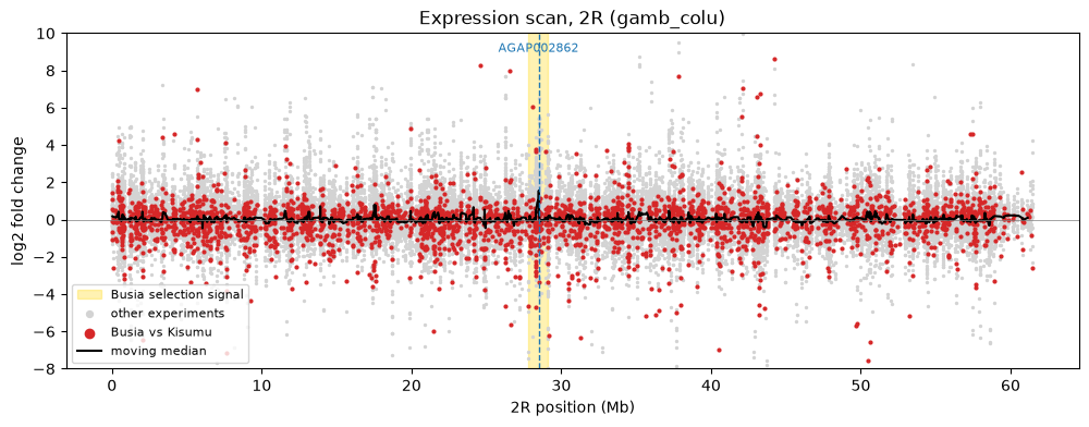
plot_scan("2R", xlim=(27, 30)) # zoom in on the Cyp6 cluster and the Busia signal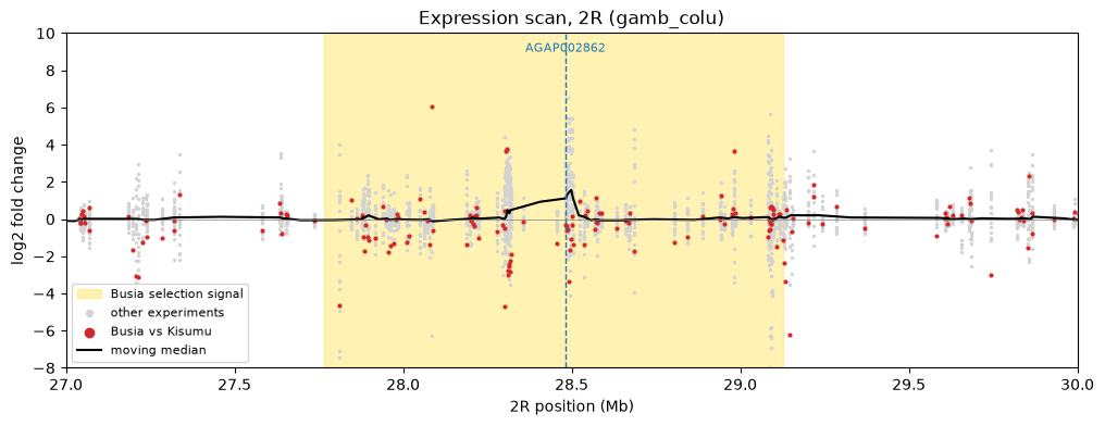
The moving median peaks at the Cyp6aa/Cyp6p cluster (about 28.5 Mb), right in the middle of the Busia selection signal. The peak is driven by the other experiments (grey). The Busia points (red) at the cluster sit below zero, while a few genes nearby, at about 28.3 Mb, are strongly up in Busia.
The scan mixes all experiments. To see what Busia does in a region, pull out the fold changes for every gene in a span and draw a heatmap. Genes are sorted by position.
AnoExpress uses compound contigs for regions: 2RL is 2R followed by 2L, and 3RL is 3R followed by
3L. Positions on 2R and 3R are the same as usual; positions on 2L and 3L are shifted by the length of 2R
(61,545,105 bp) or 3R (53,200,684 bp). region_around() below handles this for you.
def region_around(gene_id, flank=100_000):
    """Return an AnoExpress region string (compound contigs) centred on a gene."""
    g = gff.query("GeneID == @gene_id").iloc[0]
    return f"{g.contig}:{max(1, g.start - flank)}-{g.end + flank}"


def region_heatmap(region, analysis="gamb_colu"):
    df = xpress.data(
        data_type="fcs", analysis=analysis, gene_id=region,
        gff_method="malariagen_data", sort_by="position", annotations=True,
    ).reset_index()
    names = df["GeneName"].fillna("")
    # highlight the Cyp6aa/Cyp6p genes and your candidates with a marker
    mark = names.str.match(r"CYP6(AA|P)\d") | df["GeneID"].isin(CANDIDATE_GENES)
    df.index = np.where(mark, "▶ ", "") + df["GeneID"] + " " + names
    df = df.drop(columns=["GeneID", "GeneName", "GeneDescription"])
    return px.imshow(
        df, color_continuous_scale="RdBu_r", zmin=-6, zmax=6, aspect="auto",
        labels={"color": "log2FC"}, height=250 + 14 * len(df), width=900, title=region,
    )


region_heatmap("2RL:28,380,000-28,600,000") # the Cyp6aa/Cyp6p clusterThe Cyp6aa and Cyp6p genes are marked with ▶. CYP6AA1, CYP6AA2, CYP6P3 and CYP6P4 are red in most
West African experiments, which fits a regulatory or CNV mechanism spanning several genes, like the
Cyp6aa1 duplication. In the Busia column (the last one) they are white or blue. Yet this region is the centre of a strong selection signal in
Busia (Day 3). A little further out, but still inside that signal, several genes are strongly up in
Busia: AGAP002850, AGAP002852 and CYP6Z4 (AGAP002894) are all in the candidate pool.
Look closely at the six Côte d’Ivoire columns (Agboville, Dabou, Tiassale): CYP6P1 to CYP6P5 have identical fold changes. That suggests reads from these very similar genes were counted together in that study. Processing choices in the original studies carry through into any meta-analysis.
Exercise 2
Run a genome-wide expression scan for the chromosome arm that carries your first candidate gene. Is the gene in a region where many neighbours are also overexpressed?
Draw a heatmap for 100 kb either side of each of your candidates using
region_around()andregion_heatmap(). Are neighbouring genes up in Busia too?What would you look for on Day 3 to test whether a CNV explains the pattern?
Show answer
gene = CANDIDATE_GENES[0]
plot_scan(gene_arm(gene))

for gene in CANDIDATE_GENES:
    region_heatmap(region_around(gene)).show()
For GSTE4 (AGAP009193), the neighbouring epsilon GSTs (GSTE3, GSTE5, GSTE6, GSTE7) are all modestly up in Busia, while GSTE2 is down, so the whole cluster is not simply duplicated in this colony. On Day 3, check CNV frequencies in the Ugandan Ag3 cohorts at the gene (gene_cnv_frequencies()), and whether a known CNV (for example a Gstue or Cyp6aap duplication) covers it. If the duplication is common in Busia and covers all the co-expressed genes, a CNV is a good explanation.
Gene families
Most metabolic resistance genes belong to a few large families: cytochrome P450s, glutathione S-transferases (GSTs), carboxylesterases (COEs), UDP-glucuronosyltransferases (UGTs) and ABC transporters. Looking at the whole family shows whether your gene stands out from its relatives, or whether the whole family moves together.
plot_gene_family_expression() takes a Pfam domain (short name) or a GO term, and plots every
gene that carries it. Useful Pfam names from the AnoExpress notebooks:
| Family | Pfam short names |
|---|---|
| Cytochrome P450s | p450 |
| GSTs | GST_N, GST_N_3, GST_C |
| Carboxylesterases | COesterase |
| ABC transporters | ABC_membrane, ABC_tran |
| UGTs | UDPGT |
| Chemosensory proteins | OS-D |
| Odorant binding proteins | PBP_GOBP |
xpress.plot_gene_family_expression(
    gene_identifier=["GST_N", "GST_N_3", "GST_C"],
    analysis="gamb_colu",
    title="GSTs",
    sort_by="median",
    width=900,
)Co-expression
Genes that go up and down together across many experiments may share a regulator, sit on the same CNV,
or work in the same pathway. A simple way to find co-expressed genes is to correlate fold changes across
experiments. With only 18 gamb_colu comparisons the correlations are noisy, so treat the top hits as
leads, not conclusions.
The AnoExpress gene regulatory network notebook goes further, using GENIE3 to link transcription factors to their likely targets.
def coexpressed(gene_id, n=15, min_comparisons=12):
    ok = fc.notna().sum(axis=1) >= min_comparisons
    r = fc[ok].T.corrwith(fc.loc[gene_id]).drop(gene_id).dropna()
    top = r.sort_values(ascending=False).head(n).rename("pearson_r").to_frame()
    top = top.join(annots).join(gff.set_index("GeneID")[["contig", "start"]])
    top["same_region"] = (top["contig"] == gff.query("GeneID == @gene_id")["contig"].iloc[0]) & (
        (top["start"] - gff.query("GeneID == @gene_id")["start"].iloc[0]).abs() < 500_000
    )
    return top


coexpressed(CANDIDATE_GENES[0])The same_region column flags hits within 500 kb of your gene. Neighbouring genes at the top of the list
point towards a shared CNV or regulatory region.
Exercise 3
List the genes most co-expressed with each of your candidates. Are any of them known resistance genes (P450s, GSTs, COEs, Sap genes)?
Are any of the co-expressed genes physical neighbours? What does that suggest?
Plot the fold changes of your gene and its top three partners with
plot_gene_expression().
Show answer
for gene in CANDIDATE_GENES:
    display(coexpressed(gene))

top = coexpressed(CANDIDATE_GENES[0]).index[:3].to_list()
xpress.plot_gene_expression(gene_id=[CANDIDATE_GENES[0]] + top, analysis="gamb_colu", width=900, height=400)
For CYP6AA1, the top hit is its neighbour CYP6P2, and CYP6P1 is also in the top 15 (same_region is True), consistent with the cluster being regulated or duplicated as a unit. Be careful, though: part of that correlation comes from the Côte d’Ivoire studies, where CYP6P1 to CYP6P5 share identical values. Most other top hits are unrelated genes scattered around the genome with correlations above 0.9. With only 18 data points, many genes correlate strongly by chance, so use co-expression to generate hypotheses, not to confirm them.
Enrichment
Finally, zoom out. Which kinds of genes are overexpressed in Busia, and which are overexpressed consistently across experiments? A hypergeometric test asks whether a gene list contains more members of a GO term or Pfam domain than expected by chance, given how many genes carry it genome-wide. AnoExpress corrects the p-values for multiple testing (Benjamini-Hochberg).
Here we test the genes that are significantly overexpressed in at least 10 of the 18 gamb_colu comparisons.
n_up = ((fc > 0) & (padj < 0.05)).sum(axis=1)
consistent = n_up[n_up >= 10].index.to_list()
print(f"{len(consistent)} genes overexpressed in >= 10 comparisons")

pfam_enrich = xpress.pfam_hypergeometric(analysis="gamb_colu", gene_ids=consistent)
pfam_enrich.query("padj < 0.05")
235 genes overexpressed in >= 10 comparisons
Exercise 4
Repeat the Pfam enrichment for genes that are significantly overexpressed in Busia with log2FC > 2. Which gene families are enriched? Are they the same as in the consistent set?
Run a GO enrichment on the same list with
xpress.go_hypergeometric(). Which terms come up?Is your gene in an enriched family? Does that make it a stronger or a weaker candidate?
Show answer
busia_up = fc.index[(fc[BUSIA] > 2) & (padj[BUSIA] < 0.05)].to_list()
print(len(busia_up))
display(xpress.pfam_hypergeometric(analysis="gamb_colu", gene_ids=busia_up).query("padj < 0.05"))
display(xpress.go_hypergeometric(analysis="gamb_colu", gene_ids=busia_up).head(15))
The consistent set is dominated by P450s (p450). The Busia list is less clean: many of its most overexpressed genes are unannotated, and those drop out of an annotation-based test. Being in an enriched family (for example a P450) raises the prior that a gene can metabolise insecticide, but it does not make it more likely to be the causal gene in Busia. Selection (Day 3) and association with survival (Day 4) are stronger evidence.
Exercise 5: update your dossier
Write the Replication section of your gene dossier for each candidate. Include:
the Busia log2FC and adjusted p-value;
the number of
gamb_colucomparisons with significant over- and underexpression, and where they are from;whether neighbouring genes are co-overexpressed (possible CNV), and the gene’s top co-expressed partners;
your judgement: is the Busia result replicated, Busia-specific, or contradicted elsewhere?
Quiz
%pip install -q jupyterquiz==2.9.6.4
from jupyterquiz import display_quiz
display_quiz("https://raw.githubusercontent.com/sanjaynagi/anopheles-omics-training/main/quizzes/2-3-anoexpress.json")Summary
One RNA-seq experiment cannot separate resistance genes from colony differences. Replication across independent studies is a cheap, powerful filter.
AnoExpress gives comparable fold changes and adjusted p-values for many resistant vs susceptible comparisons, including Busia. It is a collection, not a pooled test: count, look and think.
Fold changes depend on the reference strain. CYP6AA1, our worked example, is up 7- to 14-fold in Côte d’Ivoire but unchanged in Busia vs Kisumu, even though it lies in the Busia 2R sweep and is duplicated on the East African triple-mutant haplotype.
Genome-wide expression scans and region heatmaps reveal clusters of co-overexpressed neighbours, which often point to CNVs, the topic of Day 3.
Gene families, co-expression and enrichment put a candidate in context, but they add prior plausibility rather than direct evidence.
Well done!
You now know whether your genes replicate. Tomorrow you ask why they are overexpressed, and whether they are under selection in wild Ugandan and Kenyan mosquitoes.
References
Nagi SC, Ingham VA. AnoExpress: Anopheles gene expression in resistance studies. Python package and Colab notebooks, https://
github .com /sanjaynagi /AnoExpress (version 0.3.3). Nagi SC, Oruni A, Weetman D, Donnelly MJ (2023). RNA-Seq-Pop: Exploiting the sequence in RNA sequencing, a Snakemake workflow reveals patterns of insecticide resistance in the malaria vector Anopheles gambiae. Molecular Ecology Resources 23: 946–961. Nagi et al. (2023)
Ingham VA, Wagstaff S, Ranson H (2018). Transcriptomic meta-signatures identified in Anopheles gambiae populations reveal previously undetected insecticide resistance mechanisms. Nature Communications 9: 5282. Ingham et al. (2018)
Ingham VA, Anthousi A, Douris V, et al. (2020). A sensory appendage protein protects malaria vectors from pyrethroids. Nature 577: 376–380. Ingham et al. (2019)
Love MI, Huber W, Anders S (2014). Moderated estimation of fold change and dispersion for RNA-seq data with DESeq2. Genome Biology 15: 550. Love et al. (2014)
Ingham VA, Morgan J, Lees RS, Ranson H (2019). Characterisation of Anopheles strains used for laboratory screening of new vector control products. Parasites & Vectors 12. Williams et al. (2019)
Njoroge H, van’t Hof A, Oruni A, et al. (2022). Identification of a rapidly-spreading triple mutant for high-level metabolic insecticide resistance in Anopheles gambiae provides a real-time molecular diagnostic for antimalarial intervention deployment. Molecular Ecology 31: 4307–4318. Njoroge et al. (2022)
- Nagi, S. C., Oruni, A., Weetman, D., & Donnelly, M. J. (2023). RNA‐Seq‐Pop : Exploiting the sequence in <scp>RNA</scp> sequencing—A Snakemake workflow reveals patterns of insecticide resistance in the malaria vector Anopheles gambiae. Molecular Ecology Resources, 23(4), 946–961. 10.1111/1755-0998.13759
- Ingham, V. A., Wagstaff, S., & Ranson, H. (2018). Transcriptomic meta-signatures identified in Anopheles gambiae populations reveal previously undetected insecticide resistance mechanisms. Nature Communications, 9(1). 10.1038/s41467-018-07615-x
- Ingham, V. A., Anthousi, A., Douris, V., Harding, N. J., Lycett, G., Morris, M., Vontas, J., & Ranson, H. (2019). A sensory appendage protein protects malaria vectors from pyrethroids. Nature, 577(7790), 376–380. 10.1038/s41586-019-1864-1
- Love, M. I., Huber, W., & Anders, S. (2014). Moderated estimation of fold change and dispersion for RNA-seq data with DESeq2. Genome Biology, 15(12). 10.1186/s13059-014-0550-8
- Williams, J., Flood, L., Praulins, G., Ingham, V. A., Morgan, J., Lees, R. S., & Ranson, H. (2019). Characterisation of Anopheles strains used for laboratory screening of new vector control products. Parasites & Vectors, 12(1). 10.1186/s13071-019-3774-3
- Njoroge, H., van’t Hof, A., Oruni, A., Pipini, D., Nagi, S. C., Lynd, A., Lucas, E. R., Tomlinson, S., Grau‐Bove, X., McDermott, D., Wat’senga, F. T., Manzambi, E. Z., Agossa, F. R., Mokuba, A., Irish, S., Kabula, B., Mbogo, C., Bargul, J., Paine, M. J. I., … Donnelly, M. J. (2022). Identification of a rapidly‐spreading triple mutant for high‐level metabolic insecticide resistance in Anopheles gambiae provides a real‐time molecular diagnostic for antimalarial intervention deployment. Molecular Ecology, 31(16), 4307–4318. 10.1111/mec.16591